13.2 A Simple Problem

Before we can continue examining MPI, we need a more interesting problem to investigate. We will begin by looking at how you might write a program to calculate the area under a curve, i.e., a numerical integration. This is a fairly standard problem for introducing parallel calculations because it can be easily decomposed into parts that can be shared among the computers in a cluster. Although in most cases it can be solved quickly on a single processor, the parallel solution illustrates all the basics you need to get started writing MPI code. We'll keep coming back to this problem in later chapters so you'll probably grow tired of it. But sticking to the same problem will make it easy for us to focus on programming constructs without getting bogged down with the details of different problems.

If you are familiar with numerical integration, you can skim this section quickly and move on to the next. Although this problem is a bit mathematical, it is straightforward and the mathematics shouldn't create much of a problem. Each step in the problem in this section is carefully explained, and you don't need to worry about every detail to get the basic idea.

13.2.1 Background

Let's get started. Suppose you are driving a car whose clock and speedometer work, but whose odometer doesn't work. How do you determine how far you have driven? If you are traveling at a constant speed, the distance traveled is the speed that you are traveling multiplied by the amount of time you travel. If you go 60 miles an hour for two hours, you travel 120 miles. If your speed is changing, you'll need to do a lot of little calculations and add up the results. For example, if you go 60 for 30 minutes, slow down to 40 for construction for the next 30 minutes, and then hotfoot it at 70 for the next hour to make up time, your total distance is 30 plus 20 plus 70 or 120 miles. You just calculate the distance traveled at each speed and add up the results.

If we plot speed against time, we can see that what we are calculating is the area under the curve. Basically, we are dividing the area into rectangles, calculating the area of each rectangle, and then adding up the results. In our example, the first rectangle has a width of one half (half an hour) and a height of 60, the second a width of one half and a height of 40, and the third a width of 1 and a height of 70. If your speed changes a lot, you will just have more rectangles. Figure 13-1 gives the basic idea.

Figure 13-1. Area is distance traveled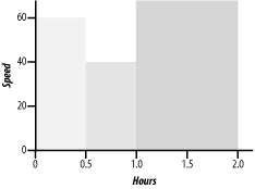

Of course, in practice, your speed will change smoothly rather than in steps so that you won't be able to fit rectangles perfectly into the area. But the area under the curve does give the exact answer to the problem, and you can approximate the area by adding up rectangles. Generally, the more rectangles you use, the better your approximation.

In Figure 13-2, three rectangles are used to estimate the area under a curve for a similar problem. In Figure 13-3, six rectangles are used. The shaded areas in each determine the error in the approximation of the total area. However, since some of these areas are above the curve and some below, they tend to cancel each other out, at least in part. Unfortunately, this is not always the case.^[1]

^[1] Those of you who remember your calculus recognize that we are calculating definite integrals. But as a numerical technique, this approximation will work even if you can't do the integration. (Ever run across an integral you couldn't evaluate?) You may also be asking why we aren't using the trapezoid rule. We are trying to keep things simple. The trapezoid rule is left as an exercise for those of you who remember it.

Figure 13-2. Approximating with three rectangles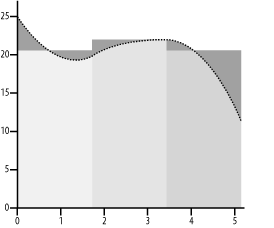

Figure 13-3. Approximating with six rectangles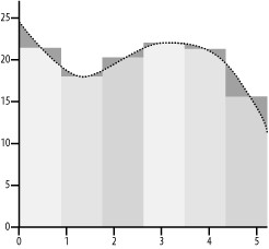

We can do this calculation without bothering to do the graph. All we need are the heights and widths of the rectangles. Widths are easy-we just divide the trip duration by however many rectangles we want. For the heights, we will need a way to calculate the speed during the rectangle. What we really want is the average speed. As an approximation, the simplest approach is to use the speed at the middle of a rectangle. For most problems of this general type, some function or rule is used to calculate this value.

Let's turn this into to a more generic problem. Suppose you want to know the area under the curve f(x) = x2 between 2 and 5. This is the shaded region in Figure 13-4, which shows what the graph of this problem would look like if we use three rectangles.

Figure 13-4. Area under x² from 2 to 5 with three rectangles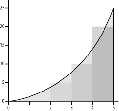

With three rectangles, the width of each will be 1. To find the height, we take the center of each rectangle (2.5, 3.5, and 4.5) and evaluate the function (2.5² = 6.25, 35² = 12.25, and 4.5² = 20.25). Multiplying height by width for each rectangle and adding the results gives an area of 38.75. (Using calculus, we know the exact answer is 39.0, so we aren't far off.)

13.2.2 Single-Processor Program

Being computer types, we'll want to write a program to do the calculation. This will allow us to easily use many more rectangles to get better results and will allow us to easily change the endpoints and functions we use. Here is the code in C:

#include <stdio.h>

   

/* problem parameters */

#define f(x)            ((x) * (x))

#define numberRects     50

#define lowerLimit      2.0

#define upperLimit      5.0

   

int main ( int argc, char * argv[  ] )

{

   int         i;

   double      area, at, height, width;

   

   area = 0.0;

   width = (upperLimit - lowerLimit) / numberRects; 

   

   for (i = 0; i < numberRects; i++)

   {  at = lowerLimit + i * width + width / 2.0;

      height = f(at);

      area = area + width * height;

   }

   

   printf("The area from %f to %f is: %f\n", lowerLimit, upperLimit, area );

   

   return 0;

}

After entering the code with our favorite text editor, we can compile and run it.

[sloanjd@cs sloanjd]$ gcc rect.c -o rect

[sloanjd@cs sloanjd]$ ./rect

The area from 2.000000 to 5.000000 is: 38.999100

This is a much better answer.

This code should be self-explanatory, but a few comments can't hurt. First, macros are used to define the problem parameters, including the function that we are looking at. For the parameters, this lets us avoid the I/O issue when we code the MPI solution. The macro for the function is used to gain the greater efficiency of inline code while maintaining the clarity of a separate function. While this isn't much of an issue here, it is good to get in the habit of using macros. The heart of the code is a loop that, for each rectangle, first calculates the height of the rectangle and then calculates the area of the rectangle, adding it to a running total. Since we want to calculate the height of the rectangle at the middle of the interval, we add width/2.0 when calculating at, the location we feed into the function. Obviously, there are a few things we can do to tighten up this code, but let's not worry about that right now