2.1 Design an experiment (i.e., design and write programs and take measurements) to determine the memory bandwidth of your computer and to estimate the caches at various levels of the hierarchy. Use this experiment to estimate the bandwidth and L1 cache of your computer. Justify your answer. (Hint: To test bandwidth, you do not want reuse. To test cache size, you want reuse to see the effect of the cache and to increase this size until the reuse decreases sharply.)
2.2 Consider a memory system with a level 1 cache of 32 KB and DRAM of 512 MB with the processor operating at 1 GHz. The latency to L1 cache is one cycle and the latency to DRAM is 100 cycles. In each memory cycle, the processor fetches four words (cache line size is four words). What is the peak achievable performance of a dot product of two vectors? Note: Where necessary, assume an optimal cache placement policy.
1        /* dot product loop */
2        for (i = 0; i < dim; i++)
3                dot_prod += a[i] * b[i];
2.3 Now consider the problem of multiplying a dense matrix with a vector using a two-loop dot-product formulation. The matrix is of dimension 4K x 4K. (Each row of the matrix takes 16 KB of storage.) What is the peak achievable performance of this technique using a two-loop dot-product based matrix-vector product?
1        /* matrix-vector product loop */
2        for (i = 0; i < dim; i++)
3                for (j = 0; i < dim; j++)
4                        c[i] += a[i][j] * b[j];
2.4 Extending this further, consider the problem of multiplying two dense matrices of dimension 4K x 4K. What is the peak achievable performance using a three-loop dot-product based formulation? (Assume that matrices are laid out in a row-major fashion.)
1        /* matrix-matrix product loop */
2        for (i = 0; i < dim; i++)
3                for (j = 0; i < dim; j++)
4                        for (k = 0; k < dim; k++)
5                                c[i][j] += a[i][k] * b[k][j];
2.5 Restructure the matrix multiplication algorithm to achieve better cache performance. The most obvious cause of the poor performance of matrix multiplication was the absence of spatial locality. In some cases, we were wasting three of the four words fetched from memory. To fix this problem, we compute the elements of the result matrix four at a time. Using this approach, we can increase our FLOP count with a simple restructuring of the program. However, it is possible to achieve much higher performance from this problem. This is possible by viewing the matrix multiplication problem as a cube in which each internal grid point corresponds to a multiply-add operation. Matrix multiplication algorithms traverse this cube in different ways, which induce different partitions of the cube. The data required for computing a partition grows as the surface area of the input faces of the partition and the computation as the volume of the partition. For the algorithms discussed above, we were slicing thin partitions of the cube for which the area and volume were comparable (thus achieving poor cache performance). To remedy this, we restructure the computation by partitioning the cube into subcubes of size k x k x k. The data associated with this is 3 x k2 (k2 data for each of the three matrices) and the computation is k3. To maximize performance, we would like 3 x k2 to be equal to 8K since that is the amount of cache available (assuming the same machine parameters as in Problem 2.2). This corresponds to k = 51. The computation associated with a cube of this dimension is 132651 multiply-add operations or 265302 FLOPs. To perform this computation, we needed to fetch two submatrices of size 51 x 51. This corresponds to 5202 words or 1301 cache lines. Accessing these cache lines takes 130100 ns. Since 265302 FLOPs are performed in 130100 ns, the peak computation rate of this formulation is 2.04 GFLOPS. Code this example and plot the performance as a function of k. (Code on any conventional microprocessor. Make sure you note the clock speed, the microprocessor and the cache available at each level.)
2.6 Consider an SMP with a distributed shared-address-space. Consider a simple cost model in which it takes 10 ns to access local cache, 100 ns to access local memory, and 400 ns to access remote memory. A parallel program is running on this machine. The program is perfectly load balanced with 80% of all accesses going to local cache, 10% to local memory, and 10% to remote memory. What is the effective memory access time for this computation? If the computation is memory bound, what is the peak computation rate?
Now consider the same computation running on one processor. Here, the processor hits the cache 70% of the time and local memory 30% of the time. What is the effective peak computation rate for one processor? What is the fractional computation rate of a processor in a parallel configuration as compared to the serial configuration?
Hint: Notice that the cache hit for multiple processors is higher than that for one processor. This is typically because the aggregate cache available on multiprocessors is larger than on single processor systems.
2.7 What are the major differences between message-passing and shared-address-space computers? Also outline the advantages and disadvantages of the two.
2.8 Why is it difficult to construct a true shared-memory computer? What is the minimum number of switches for connecting p processors to a shared memory with b words (where each word can be accessed independently)?
2.9 Of the four PRAM models (EREW, CREW, ERCW, and CRCW), which model is the most powerful? Why?
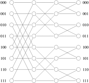
2.10 [Lei92] The Butterfly network is an interconnection network composed of log p levels (as the omega network). In a Butterfly network, each switching node i at a level l is connected to the identically numbered element at level l + 1 and to a switching node whose number differs from itself only at the lth most significant bit. Therefore, switching node Si is connected to element S j at level l if j = i or j = i  (2log p-l ).
Figure 2.34 illustrates a Butterfly network with eight processing nodes. Show the equivalence of a Butterfly network and an omega network.

Hint: Rearrange the switches of an omega network so that it looks like a Butterfly network.
2.11 Consider the omega network described in Section 2.4.3. As shown there, this network is a blocking network (that is, a processor that uses the network to access a memory location might prevent another processor from accessing another memory location). Consider an omega network that connects p processors. Define a function f that maps P = [0, 1, ..., p - 1] onto a permutation P' of P (that is, P'[i] = f(P[i]) and P'[i]  P for all 0
  i < p). Think of this function as mapping communication requests by the processors so that processor P[i] requests communication with processor P'[i].
How many distinct permutation functions exist?
How many of these functions result in non-blocking communication?
What is the probability that an arbitrary function will result in non-blocking communication?
2.12 A cycle in a graph is defined as a path originating and terminating at the same node. The length of a cycle is the number of edges in the cycle. Show that there are no odd-length cycles in a d-dimensional hypercube.
2.13 The labels in a d-dimensional hypercube use d bits. Fixing any k of these bits, show that the nodes whose labels differ in the remaining d - k bit positions form a (d - k)-dimensional subcube composed of 2(d-k) nodes.
2.14 Let A and B be two nodes in a d-dimensional hypercube. Define H(A, B) to be the Hamming distance between A and B, and P(A, B) to be the number of distinct paths connecting A and B. These paths are called parallel paths and have no common nodes other than A and B. Prove the following:
The minimum distance in terms of communication links between A and B is given by H(A, B).
The total number of parallel paths between any two nodes is P(A, B) = d .
The number of parallel paths between A and B of length H(A, B) is Plength=H(A,B)(A, B) = H(A, B).
The length of the remaining d - H(A, B) parallel paths is H(A, B) + 2.
2.15 In the informal derivation of the bisection width of a hypercube, we used the construction of a hypercube to show that a d-dimensional hypercube is formed from two (d - 1)-dimensional hypercubes. We argued that because corresponding nodes in each of these subcubes have a direct communication link, there are 2d - 1 links across the partition. However, it is possible to partition a hypercube into two parts such that neither of the partitions is a hypercube. Show that any such partitions will have more than 2d - 1 direct links between them.
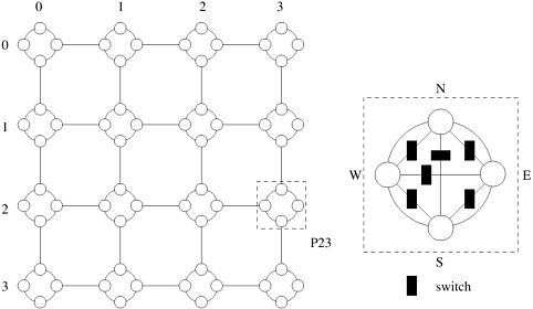
2.16 [MKRS88] A  reconfigurable mesh consists of a
  array of processing nodes connected to a grid-shaped reconfigurable broadcast bus. A 4 x 4 reconfigurable mesh is shown in Figure 2.35. Each node has locally-controllable bus switches. The internal connections among the four ports, north (N), east (E), west (W), and south (S), of a node can be configured during the execution of an algorithm. Note that there are 15 connection patterns. For example, {SW, EN} represents the configuration in which port S is connected to port W and port N is connected to port E. Each bit of the bus carries one of 1-signal or 0-signal at any time. The switches allow the broadcast bus to be divided into subbuses, providing smaller reconfigurable meshes. For a given set of switch settings, a subbus is a maximally-connected subset of the nodes. Other than the buses and the switches, the reconfigurable mesh is similar to the standard two-dimensional mesh. Assume that only one node is allowed to broadcast on a subbus shared by multiple nodes at any time.

Determine the bisection width, the diameter, and the number of switching nodes and communication links for a reconfigurable mesh of  processing nodes. What are the advantages and disadvantages of a reconfigurable mesh as compared to a wraparound mesh?
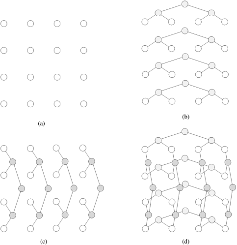
2.17 [Lei92] A mesh of trees is a network that imposes a tree interconnection on a grid of processing nodes. A  mesh of trees is constructed as follows. Starting with a
  grid, a complete binary tree is imposed on each row of the grid. Then a complete binary tree is imposed on each column of the grid. Figure 2.36 illustrates the construction of a 4 x 4 mesh of trees. Assume that the nodes at intermediate levels are switching nodes. Determine the bisection width, diameter, and total number of switching nodes in a
  mesh.
mesh.

2.18 [Lei92] Extend the two-dimensional mesh of trees (Problem 2.17) to d dimensions to construct a p1/d x p1/d x ··· x p1/d mesh of trees. We can do this by fixing grid positions in all dimensions to different values and imposing a complete binary tree on the one dimension that is being varied.
Derive the total number of switching nodes in a p1/d x p1/d x ··· x p1/d mesh of trees. Calculate the diameter, bisection width, and wiring cost in terms of the total number of wires. What are the advantages and disadvantages of a mesh of trees as compared to a wraparound mesh?
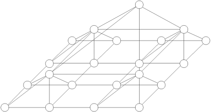
2.19 [Lei92] A network related to the mesh of trees is the d-dimensional pyramidal mesh. A d-dimensional pyramidal mesh imposes a pyramid on the underlying grid of processing nodes (as opposed to a complete tree in the mesh of trees). The generalization is as follows. In the mesh of trees, all dimensions except one are fixed and a tree is imposed on the remaining dimension. In a pyramid, all but two dimensions are fixed and a pyramid is imposed on the mesh formed by these two dimensions. In a tree, each node i at level k is connected to node i/2 at level k - 1. Similarly, in a pyramid, a node (i, j) at level k is connected to a node (i/2, j/2) at level k - 1. Furthermore, the nodes at each level are connected in a mesh. A two-dimensional pyramidal mesh is illustrated in Figure 2.37.

For a  pyramidal mesh, assume that the intermediate nodes are switching nodes, and derive the diameter, bisection width, arc connectivity, and cost in terms of the number of communication links and switching nodes. What are the advantages and disadvantages of a pyramidal mesh as compared to a mesh of trees?
2.20 [Lei92] One of the drawbacks of a hypercube-connected network is that different wires in the network are of different lengths. This implies that data takes different times to traverse different communication links. It appears that two-dimensional mesh networks with wraparound connections suffer from this drawback too. However, it is possible to fabricate a two-dimensional wraparound mesh using wires of fixed length. Illustrate this layout by drawing such a 4 x 4 wraparound mesh.
2.21 Show how to embed a p-node three-dimensional mesh into a p-node hypercube. What are the allowable values of p for your embedding?
2.22 Show how to embed a p-node mesh of trees into a p-node hypercube.
2.23 Consider a complete binary tree of 2d - 1 nodes in which each node is a processing node. What is the minimum-dilation mapping of such a tree onto a d-dimensional hypercube?
2.24 The concept of a minimum congestion mapping is very useful. Consider two parallel computers with different interconnection networks such that a congestion-r mapping of the first into the second exists. Ignoring the dilation of the mapping, if each communication link in the second computer is more than r times faster than the first computer, the second computer is strictly superior to the first.
Now consider mapping a d-dimensional hypercube onto a 2d-node mesh. Ignoring the dilation of the mapping, what is the minimum-congestion mapping of the hypercube onto the mesh? Use this result to determine whether a 1024-node mesh with communication links operating at 25 million bytes per second is strictly better than a 1024-node hypercube (whose nodes are identical to those used in the mesh) with communication links operating at two million bytes per second.
2.25 Derive the diameter, number of links, and bisection width of a k-ary d-cube with p nodes. Define lav to be the average distance between any two nodes in the network. Derive lav for a k-ary d-cube.
2.26 Consider the routing of messages in a parallel computer that uses store-and-forward routing. In such a network, the cost of sending a single message of size m from Psource to Pdestination via a path of length d is ts + tw x d x m. An alternate way of sending a message of size m is as follows. The user breaks the message into k parts each of size m/k, and then sends these k distinct messages one by one from Psource to Pdestination. For this new method, derive the expression for time to transfer a message of size m to a node d hops away under the following two cases:
Assume that another message can be sent from Psource as soon as the previous message has reached the next node in the path.
Assume that another message can be sent from Psource only after the previous message has reached Pdestination.
For each case, comment on the value of this expression as the value of k varies between 1 and m. Also, what is the optimal value of k if ts is very large, or if ts = 0?
2.27 Consider a hypercube network of p nodes. Assume that the channel width of each communication link is one. The channel width of the links in a k-ary d-cube (for d < log p) can be increased by equating the cost of this network with that of a hypercube. Two distinct measures can be used to evaluate the cost of a network.
The cost can be expressed in terms of the total number of wires in the network (the total number of wires is a product of the number of communication links and the channel width).
The bisection bandwidth can be used as a measure of cost.
Using each of these cost metrics and equating the cost of a k-ary d-cube with a hypercube, what is the channel width of a k-ary d-cube with an identical number of nodes, channel rate, and cost?
2.28 The results from Problems 2.25 and 2.27 can be used in a cost-performance analysis of static interconnection networks. Consider a k-ary d-cube network of p nodes with cut-through routing. Assume a hypercube-connected network of p nodes with channel width one. The channel width of other networks in the family is scaled up so that their cost is identical to that of the hypercube. Let s and s' be the scaling factors for the channel width derived by equating the costs specified by the two cost metrics in Problem 2.27.
For each of the two scaling factors s and s', express the average communication time between any two nodes as a function of the dimensionality (d)of a k-ary d-cube and the number of nodes. Plot the communication time as a function of the dimensionality for p = 256, 512, and 1024, message size m = 512 bytes, ts = 50.0µs, and th = tw = 0.5µs (for the hypercube). For these values of p and m, what is the dimensionality of the network that yields the best performance for a given cost?
2.29 Repeat Problem 2.28 for a k-ary d-cube with store-and-forward routing.