3.1 Preliminaries

Dividing a computation into smaller computations and assigning them to different processors for parallel execution are the two key steps in the design of parallel algorithms. In this section, we present some basic terminology and introduce these two key steps in parallel algorithm design using matrix-vector multiplication and database query processing as examples.

3.1.1 Decomposition, Tasks, and Dependency Graphs

The process of dividing a computation into smaller parts, some or all of which may potentially be executed in parallel, is called decomposition. Tasks are programmer-defined units of computation into which the main computation is subdivided by means of decomposition. Simultaneous execution of multiple tasks is the key to reducing the time required to solve the entire problem. Tasks can be of arbitrary size, but once defined, they are regarded as indivisible units of computation. The tasks into which a problem is decomposed may not all be of the same size.

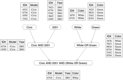
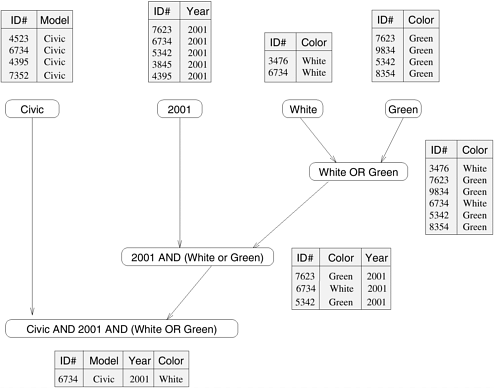
Note that all tasks in Figure 3.1 are independent and can be performed all together or in any sequence. However, in general, some tasks may use data produced by other tasks and thus may need to wait for these tasks to finish execution. An abstraction used to express such dependencies among tasks and their relative order of execution is known as a task-dependency graph. A task-dependency graph is a directed acyclic graph in which the nodes represent tasks and the directed edges indicate the dependencies amongst them. The task corresponding to a node can be executed when all tasks connected to this node by incoming edges have completed. Note that task-dependency graphs can be disconnected and the edge-set of a task-dependency graph can be empty. This is the case for matrix-vector multiplication, where each task computes a subset of the entries of the product vector. To see a more interesting task-dependency graph, consider the following database query processing example.

The various computations involved in processing the query in Example 3.2 can be visualized by the task-dependency graph shown in Figure 3.2. Each node in this figure is a task that corresponds to an intermediate table that needs to be computed and the arrows between nodes indicate dependencies between the tasks. For example, before we can compute the table that corresponds to the 2001 Civics, we must first compute the table of all the Civics and a table of all the 2001-model cars.

Note that often there are multiple ways of expressing certain computations, especially those involving associative operators such as addition, multiplication, and logical AND or OR. Different ways of arranging computations can lead to different task-dependency graphs with different characteristics. For instance, the database query in Example 3.2 can be solved by first computing a table of all green or white cars, then performing an intersection with a table of all 2001 model cars, and finally combining the results with the table of all Civics. This sequence of computation results in the task-dependency graph shown in Figure 3.3.

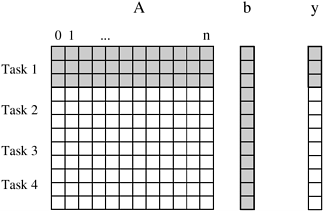
3.1.2 Granularity, Concurrency, and Task-Interaction

The number and size of tasks into which a problem is decomposed determines the granularity of the decomposition. A decomposition into a large number of small tasks is called fine-grained and a decomposition into a small number of large tasks is called coarse-grained. For example, the decomposition for matrix-vector multiplication shown in Figure 3.1 would usually be considered fine-grained because each of a large number of tasks performs a single dot-product. Figure 3.4 shows a coarse-grained decomposition of the same problem into four tasks, where each tasks computes n/4 of the entries of the output vector of length n.

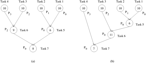
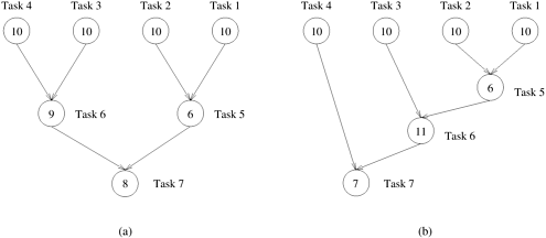
A concept related to granularity is that of degree of concurrency. The maximum number of tasks that can be executed simultaneously in a parallel program at any given time is known as its maximum degree of concurrency. In most cases, the maximum degree of concurrency is less than the total number of tasks due to dependencies among the tasks. For example, the maximum degree of concurrency in the task-graphs of Figures 3.2 and 3.3 is four. In these task-graphs, maximum concurrency is available right at the beginning when tables for Model, Year, Color Green, and Color White can be computed simultaneously. In general, for task-dependency graphs that are trees, the maximum degree of concurrency is always equal to the number of leaves in the tree.

A more useful indicator of a parallel program's performance is the average degree of concurrency, which is the average number of tasks that can run concurrently over the entire duration of execution of the program.

Both the maximum and the average degrees of concurrency usually increase as the granularity of tasks becomes smaller (finer). For example, the decomposition of matrix-vector multiplication shown in Figure 3.1 has a fairly small granularity and a large degree of concurrency. The decomposition for the same problem shown in Figure 3.4 has a larger granularity and a smaller degree of concurrency.

The degree of concurrency also depends on the shape of the task-dependency graph and the same granularity, in general, does not guarantee the same degree of concurrency. For example, consider the two task graphs in Figure 3.5, which are abstractions of the task graphs of Figures 3.2 and 3.3, respectively (Problem 3.1). The number inside each node represents the amount of work required to complete the task corresponding to that node. The average degree of concurrency of the task graph in Figure 3.5(a) is 2.33 and that of the task graph in Figure 3.5(b) is 1.88 (Problem 3.1), although both task-dependency graphs are based on the same decomposition.

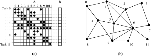
A feature of a task-dependency graph that determines the average degree of concurrency for a given granularity is its critical path. In a task-dependency graph, let us refer to the nodes with no incoming edges by start nodes and the nodes with no outgoing edges by finish nodes. The longest directed path between any pair of start and finish nodes is known as the critical path. The sum of the weights of nodes along this path is known as the critical path length, where the weight of a node is the size or the amount of work associated with the corresponding task. The ratio of the total amount of work to the critical-path length is the average degree of concurrency. Therefore, a shorter critical path favors a higher degree of concurrency. For example, the critical path length is 27 in the task-dependency graph shown in Figure 3.5(a) and is 34 in the task-dependency graph shown in Figure 3.5(b). Since the total amount of work required to solve the problems using the two decompositions is 63 and 64, respectively, the average degree of concurrency of the two task-dependency graphs is 2.33 and 1.88, respectively.

Although it may appear that the time required to solve a problem can be reduced simply by increasing the granularity of decomposition and utilizing the resulting concurrency to perform more and more tasks in parallel, this is not the case in most practical scenarios. Usually, there is an inherent bound on how fine-grained a decomposition a problem permits. For instance, there are n² multiplications and additions in matrix-vector multiplication considered in Example 3.1 and the problem cannot be decomposed into more than O(n²) tasks even by using the most fine-grained decomposition.

Other than limited granularity and degree of concurrency, there is another important practical factor that limits our ability to obtain unbounded speedup (ratio of serial to parallel execution time) from parallelization. This factor is the interaction among tasks running on different physical processors. The tasks that a problem is decomposed into often share input, output, or intermediate data. The dependencies in a task-dependency graph usually result from the fact that the output of one task is the input for another. For example, in the database query example, tasks share intermediate data; the table generated by one task is often used by another task as input. Depending on the definition of the tasks and the parallel programming paradigm, there may be interactions among tasks that appear to be independent in a task-dependency graph. For example, in the decomposition for matrix-vector multiplication, although all tasks are independent, they all need access to the entire input vector b. Since originally there is only one copy of the vector b, tasks may have to send and receive messages for all of them to access the entire vector in the distributed-memory paradigm.

The pattern of interaction among tasks is captured by what is known as a task-interaction graph. The nodes in a task-interaction graph represent tasks and the edges connect tasks that interact with each other. The nodes and edges of a task-interaction graph can be assigned weights proportional to the amount of computation a task performs and the amount of interaction that occurs along an edge, if this information is known. The edges in a task-interaction graph are usually undirected, but directed edges can be used to indicate the direction of flow of data, if it is unidirectional. The edge-set of a task-interaction graph is usually a superset of the edge-set of the task-dependency graph. In the database query example discussed earlier, the task-interaction graph is the same as the task-dependency graph. We now give an example of a more interesting task-interaction graph that results from the problem of sparse matrix-vector multiplication.

Chapter 5 contains detailed quantitative analysis of overheads due to interaction and limited concurrency and their effect on the performance and scalability of parallel algorithm-architecture combinations. In this section, we have provided a basic introduction to these factors because they require important consideration in designing parallel algorithms.

3.1.3 Processes and Mapping

The tasks, into which a problem is decomposed, run on physical processors. However, for reasons that we shall soon discuss, we will use the term process in this chapter to refer to a processing or computing agent that performs tasks. In this context, the term process does not adhere to the rigorous operating system definition of a process. Instead, it is an abstract entity that uses the code and data corresponding to a task to produce the output of that task within a finite amount of time after the task is activated by the parallel program. During this time, in addition to performing computations, a process may synchronize or communicate with other processes, if needed. In order to obtain any speedup over a sequential implementation, a parallel program must have several processes active simultaneously, working on different tasks. The mechanism by which tasks are assigned to processes for execution is called mapping. For example, four processes could be assigned the task of computing one submatrix of C each in the matrix-multiplication computation of Example 3.5.

The task-dependency and task-interaction graphs that result from a choice of decomposition play an important role in the selection of a good mapping for a parallel algorithm. A good mapping should seek to maximize the use of concurrency by mapping independent tasks onto different processes, it should seek to minimize the total completion time by ensuring that processes are available to execute the tasks on the critical path as soon as such tasks become executable, and it should seek to minimize interaction among processes by mapping tasks with a high degree of mutual interaction onto the same process. In most nontrivial parallel algorithms, these tend to be conflicting goals. For instance, the most efficient decomposition-mapping combination is a single task mapped onto a single process. It wastes no time in idling or interacting, but achieves no speedup either. Finding a balance that optimizes the overall parallel performance is the key to a successful parallel algorithm. Therefore, mapping of tasks onto processes plays an important role in determining how efficient the resulting parallel algorithm is. Even though the degree of concurrency is determined by the decomposition, it is the mapping that determines how much of that concurrency is actually utilized, and how efficiently.

For example, Figure 3.7 shows efficient mappings for the decompositions and the task-interaction graphs of Figure 3.5 onto four processes. Note that, in this case, a maximum of four processes can be employed usefully, although the total number of tasks is seven. This is because the maximum degree of concurrency is only four. The last three tasks can be mapped arbitrarily among the processes to satisfy the constraints of the task-dependency graph. However, it makes more sense to map the tasks connected by an edge onto the same process because this prevents an inter-task interaction from becoming an inter-processes interaction. For example, in Figure 3.7(b), if Task 5 is mapped onto process P₂, then both processes P₀ and P₁ will need to interact with P₂. In the current mapping, only a single interaction between P₀ and P₁ suffices.

3.1.4 Processes versus Processors

In the context of parallel algorithm design, processes are logical computing agents that perform tasks. Processors are the hardware units that physically perform computations. In this text, we choose to express parallel algorithms and programs in terms of processes. In most cases, when we refer to processes in the context of a parallel algorithm, there is a one-to-one correspondence between processes and processors and it is appropriate to assume that there are as many processes as the number of physical CPUs on the parallel computer. However, sometimes a higher level of abstraction may be required to express a parallel algorithm, especially if it is a complex algorithm with multiple stages or with different forms of parallelism.

Treating processes and processors separately is also useful when designing parallel programs for hardware that supports multiple programming paradigms. For instance, consider a parallel computer that consists of multiple computing nodes that communicate with each other via message passing. Now each of these nodes could be a shared-address-space module with multiple CPUs. Consider implementing matrix multiplication on such a parallel computer. The best way to design a parallel algorithm is to do so in two stages. First, develop a decomposition and mapping strategy suitable for the message-passing paradigm and use this to exploit parallelism among the nodes. Each task that the original matrix multiplication problem decomposes into is a matrix multiplication computation itself. The next step is to develop a decomposition and mapping strategy suitable for the shared-memory paradigm and use this to implement each task on the multiple CPUs of a node.