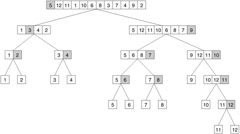
3.2 Decomposition Techniques

As mentioned earlier, one of the fundamental steps that we need to undertake to solve a problem in parallel is to split the computations to be performed into a set of tasks for concurrent execution defined by the task-dependency graph. In this section, we describe some commonly used decomposition techniques for achieving concurrency. This is not an exhaustive set of possible decomposition techniques. Also, a given decomposition is not always guaranteed to lead to the best parallel algorithm for a given problem. Despite these shortcomings, the decomposition techniques described in this section often provide a good starting point for many problems and one or a combination of these techniques can be used to obtain effective decompositions for a large variety of problems.

These techniques are broadly classified as recursive decomposition, data-decomposition, exploratory decomposition, and speculative decomposition. The recursive- and data-decomposition techniques are relatively general purpose as they can be used to decompose a wide variety of problems. On the other hand, speculative- and exploratory-decomposition techniques are more of a special purpose nature because they apply to specific classes of problems.

3.2.1 Recursive Decomposition

Recursive decomposition is a method for inducing concurrency in problems that can be solved using the divide-and-conquer strategy. In this technique, a problem is solved by first dividing it into a set of independent subproblems. Each one of these subproblems is solved by recursively applying a similar division into smaller subproblems followed by a combination of their results. The divide-and-conquer strategy results in natural concurrency, as different subproblems can be solved concurrently.

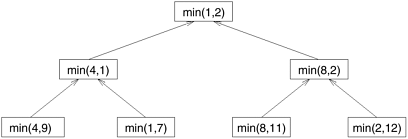
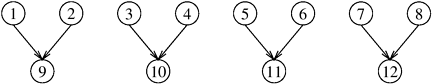
In Figure 3.8, we define a task as the work of partitioning a given subsequence. Therefore, Figure 3.8 also represents the task graph for the problem. Initially, there is only one sequence (i.e., the root of the tree), and we can use only a single process to partition it. The completion of the root task results in two subsequences (A₀ and A₁, corresponding to the two nodes at the first level of the tree) and each one can be partitioned in parallel. Similarly, the concurrency continues to increase as we move down the tree.

Sometimes, it is possible to restructure a computation to make it amenable to recursive decomposition even if the commonly used algorithm for the problem is not based on the divide-and-conquer strategy. For example, consider the problem of finding the minimum element in an unordered sequence A of n elements. The serial algorithm for solving this problem scans the entire sequence A, recording at each step the minimum element found so far as illustrated in Algorithm 3.1. It is easy to see that this serial algorithm exhibits no concurrency.

Algorithm 3.1 A serial program for finding the minimum in an array of numbers A of length n.

1.   procedure SERIAL_MIN (A, n) 
2.   begin 
3.   min = A[0]; 
4.   for i := 1 to n - 1 do 
5.       if (A[i] < min) min := A[i]; 
6.   endfor; 
7.   return min; 
8.   end SERIAL_MIN 

Once we restructure this computation as a divide-and-conquer algorithm, we can use recursive decomposition to extract concurrency. Algorithm 3.2 is a divide-and-conquer algorithm for finding the minimum element in an array. In this algorithm, we split the sequence A into two subsequences, each of size n/2, and we find the minimum for each of these subsequences by performing a recursive call. Now the overall minimum element is found by selecting the minimum of these two subsequences. The recursion terminates when there is only one element left in each subsequence. Having restructured the serial computation in this manner, it is easy to construct a task-dependency graph for this problem. Figure 3.9 illustrates such a task-dependency graph for finding the minimum of eight numbers where each task is assigned the work of finding the minimum of two numbers.

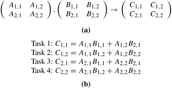
Algorithm 3.2 A recursive program for finding the minimum in an array of numbers A of length n.

1.   procedure RECURSIVE_MIN (A, n) 
2.   begin 
3.   if (n = 1) then 
4.       min := A[0]; 
5.   else 
6.       lmin := RECURSIVE_MIN (A, n/2); 
7.       rmin := RECURSIVE_MIN (&(A[n/2]), n - n/2); 
8.       if (lmin < rmin) then 
9.           min := lmin; 
10.      else 
11.          min := rmin; 
12.      endelse; 
13.  endelse; 
14.  return min; 
15.  end RECURSIVE_MIN 

3.2.2 Data Decomposition

Data decomposition is a powerful and commonly used method for deriving concurrency in algorithms that operate on large data structures. In this method, the decomposition of computations is done in two steps. In the first step, the data on which the computations are performed is partitioned, and in the second step, this data partitioning is used to induce a partitioning of the computations into tasks. The operations that these tasks perform on different data partitions are usually similar (e.g., matrix multiplication introduced in Example 3.5) or are chosen from a small set of operations (e.g., LU factorization introduced in Example 3.10).

The partitioning of data can be performed in many possible ways as discussed next. In general, one must explore and evaluate all possible ways of partitioning the data and determine which one yields a natural and efficient computational decomposition.

Partitioning Output Data In many computations, each element of the output can be computed independently of others as a function of the input. In such computations, a partitioning of the output data automatically induces a decomposition of the problems into tasks, where each task is assigned the work of computing a portion of the output. We introduce the problem of matrix-multiplication in Example 3.5 to illustrate a decomposition based on partitioning output data.

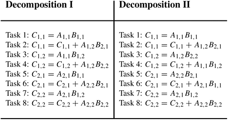
Most matrix algorithms, including matrix-vector and matrix-matrix multiplication, can be formulated in terms of block matrix operations. In such a formulation, the matrix is viewed as composed of blocks or submatrices and the scalar arithmetic operations on its elements are replaced by the equivalent matrix operations on the blocks. The results of the element and the block versions of the algorithm are mathematically equivalent (Problem 3.10). Block versions of matrix algorithms are often used to aid decomposition.

The decomposition shown in Figure 3.10 is based on partitioning the output matrix C into four submatrices and each of the four tasks computes one of these submatrices. The reader must note that data-decomposition is distinct from the decomposition of the computation into tasks. Although the two are often related and the former often aids the latter, a given data-decomposition does not result in a unique decomposition into tasks. For example, Figure 3.11 shows two other decompositions of matrix multiplication, each into eight tasks, corresponding to the same data-decomposition as used in Figure 3.10(a).

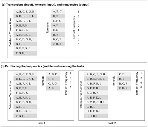
We now introduce another example to illustrate decompositions based on data partitioning. Example 3.6 describes the problem of computing the frequency of a set of itemsets in a transaction database, which can be decomposed based on the partitioning of output data.

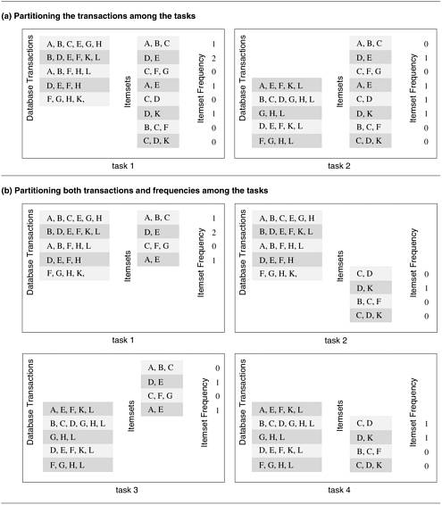
Figure 3.12(b) shows how the computation of frequencies of the itemsets can be decomposed into two tasks by partitioning the output into two parts and having each task compute its half of the frequencies. Note that, in the process, the itemsets input has also been partitioned, but the primary motivation for the decomposition of Figure 3.12(b) is to have each task independently compute the subset of frequencies assigned to it.

Partitioning Input Data Partitioning of output data can be performed only if each output can be naturally computed as a function of the input. In many algorithms, it is not possible or desirable to partition the output data. For example, while finding the minimum, maximum, or the sum of a set of numbers, the output is a single unknown value. In a sorting algorithm, the individual elements of the output cannot be efficiently determined in isolation. In such cases, it is sometimes possible to partition the input data, and then use this partitioning to induce concurrency. A task is created for each partition of the input data and this task performs as much computation as possible using these local data. Note that the solutions to tasks induced by input partitions may not directly solve the original problem. In such cases, a follow-up computation is needed to combine the results. For example, while finding the sum of a sequence of N numbers using p processes (N > p), we can partition the input into p subsets of nearly equal sizes. Each task then computes the sum of the numbers in one of the subsets. Finally, the p partial results can be added up to yield the final result.

The problem of computing the frequency of a set of itemsets in a transaction database described in Example 3.6 can also be decomposed based on a partitioning of input data. Figure 3.13(a) shows a decomposition based on a partitioning of the input set of transactions. Each of the two tasks computes the frequencies of all the itemsets in its respective subset of transactions. The two sets of frequencies, which are the independent outputs of the two tasks, represent intermediate results. Combining the intermediate results by pairwise addition yields the final result.

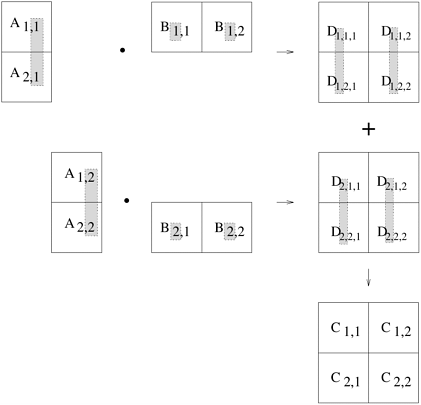
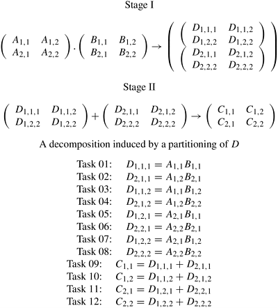
Partitioning both Input and Output Data In some cases, in which it is possible to partition the output data, partitioning of input data can offer additional concurrency. For example, consider the 4-way decomposition shown in Figure 3.13(b) for computing itemset frequencies. Here, both the transaction set and the frequencies are divided into two parts and a different one of the four possible combinations is assigned to each of the four tasks. Each task then computes a local set of frequencies. Finally, the outputs of Tasks 1 and 3 are added together, as are the outputs of Tasks 2 and 4.

Partitioning Intermediate Data Algorithms are often structured as multi-stage computations such that the output of one stage is the input to the subsequent stage. A decomposition of such an algorithm can be derived by partitioning the input or the output data of an intermediate stage of the algorithm. Partitioning intermediate data can sometimes lead to higher concurrency than partitioning input or output data. Often, the intermediate data are not generated explicitly in the serial algorithm for solving the problem and some restructuring of the original algorithm may be required to use intermediate data partitioning to induce a decomposition.

Let us revisit matrix multiplication to illustrate a decomposition based on partitioning intermediate data. Recall that the decompositions induced by a 2 x 2 partitioning of the output matrix C, as shown in Figures 3.10 and 3.11, have a maximum degree of concurrency of four. We can increase the degree of concurrency by introducing an intermediate stage in which eight tasks compute their respective product submatrices and store the results in a temporary three-dimensional matrix D, as shown in Figure 3.14. The submatrix D_k,i,j is the product of A_i,k and B_k,j.

A partitioning of the intermediate matrix D induces a decomposition into eight tasks. Figure 3.15 shows this decomposition. After the multiplication phase, a relatively inexpensive matrix addition step can compute the result matrix C. All submatrices D_*,i,j with the same second and third dimensions i and j are added to yield C_i,j. The eight tasks numbered 1 through 8 in Figure 3.15 perform O(n³/8) work each in multiplying n/2 x n/2 submatrices of A and B. Then, four tasks numbered 9 through 12 spend O(n²/4) time each in adding the appropriate n/2 x n/2 submatrices of the intermediate matrix D to yield the final result matrix C. Figure 3.16 shows the task-dependency graph corresponding to the decomposition shown in Figure 3.15.

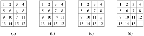
Note that all elements of D are computed implicitly in the original decomposition shown in Figure 3.11, but are not explicitly stored. By restructuring the original algorithm and by explicitly storing D, we have been able to devise a decomposition with higher concurrency. This, however, has been achieved at the cost of extra aggregate memory usage.

The Owner-Computes Rule A decomposition based on partitioning output or input data is also widely referred to as the owner-computes rule. The idea behind this rule is that each partition performs all the computations involving data that it owns. Depending on the nature of the data or the type of data-partitioning, the owner-computes rule may mean different things. For instance, when we assign partitions of the input data to tasks, then the owner-computes rule means that a task performs all the computations that can be done using these data. On the other hand, if we partition the output data, then the owner-computes rule means that a task computes all the data in the partition assigned to it.

3.2.3 Exploratory Decomposition

Exploratory decomposition is used to decompose problems whose underlying computations correspond to a search of a space for solutions. In exploratory decomposition, we partition the search space into smaller parts, and search each one of these parts concurrently, until the desired solutions are found. For an example of exploratory decomposition, consider the 15-puzzle problem.

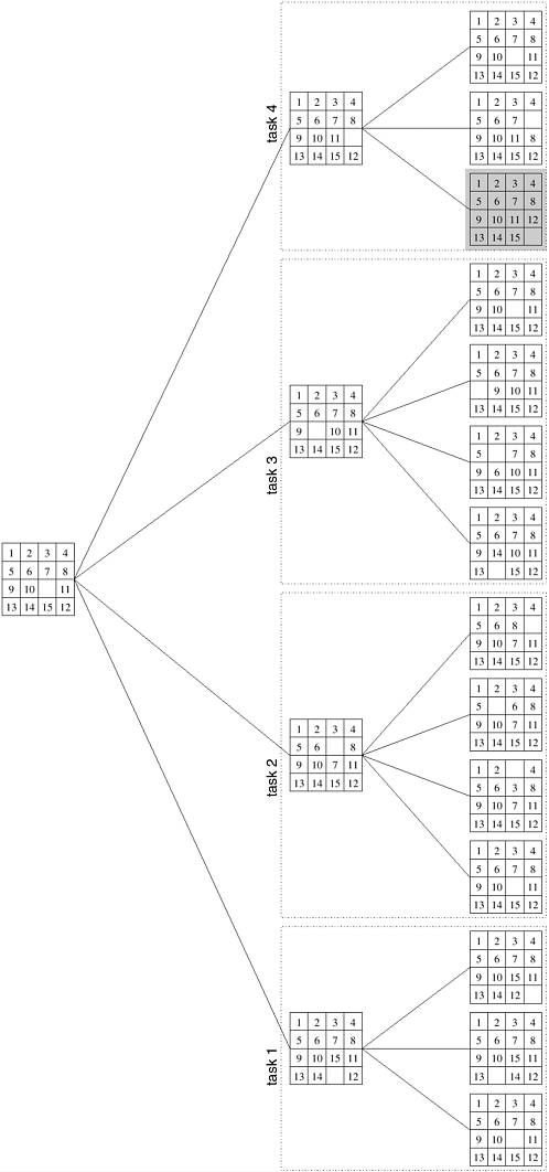
The 15-puzzle is typically solved using tree-search techniques. Starting from the initial configuration, all possible successor configurations are generated. A configuration may have 2, 3, or 4 possible successor configurations, each corresponding to the occupation of the empty slot by one of its neighbors. The task of finding a path from initial to final configuration now translates to finding a path from one of these newly generated configurations to the final configuration. Since one of these newly generated configurations must be closer to the solution by one move (if a solution exists), we have made some progress towards finding the solution. The configuration space generated by the tree search is often referred to as a state space graph. Each node of the graph is a configuration and each edge of the graph connects configurations that can be reached from one another by a single move of a tile.

One method for solving this problem in parallel is as follows. First, a few levels of configurations starting from the initial configuration are generated serially until the search tree has a sufficient number of leaf nodes (i.e., configurations of the 15-puzzle). Now each node is assigned to a task to explore further until at least one of them finds a solution. As soon as one of the concurrent tasks finds a solution it can inform the others to terminate their searches. Figure 3.18 illustrates one such decomposition into four tasks in which task 4 finds the solution.

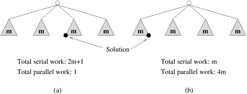
Note that even though exploratory decomposition may appear similar to data-decomposition (the search space can be thought of as being the data that get partitioned) it is fundamentally different in the following way. The tasks induced by data-decomposition are performed in their entirety and each task performs useful computations towards the solution of the problem. On the other hand, in exploratory decomposition, unfinished tasks can be terminated as soon as an overall solution is found. Hence, the portion of the search space searched (and the aggregate amount of work performed) by a parallel formulation can be very different from that searched by a serial algorithm. The work performed by the parallel formulation can be either smaller or greater than that performed by the serial algorithm. For example, consider a search space that has been partitioned into four concurrent tasks as shown in Figure 3.19. If the solution lies right at the beginning of the search space corresponding to task 3 (Figure 3.19(a)), then it will be found almost immediately by the parallel formulation. The serial algorithm would have found the solution only after performing work equivalent to searching the entire space corresponding to tasks 1 and 2. On the other hand, if the solution lies towards the end of the search space corresponding to task 1 (Figure 3.19(b)), then the parallel formulation will perform almost four times the work of the serial algorithm and will yield no speedup.

3.2.4 Speculative Decomposition

Speculative decomposition is used when a program may take one of many possible computationally significant branches depending on the output of other computations that precede it. In this situation, while one task is performing the computation whose output is used in deciding the next computation, other tasks can concurrently start the computations of the next stage. This scenario is similar to evaluating one or more of the branches of a switch statement in C in parallel before the input for the switch is available. While one task is performing the computation that will eventually resolve the switch, other tasks could pick up the multiple branches of the switch in parallel. When the input for the switch has finally been computed, the computation corresponding to the correct branch would be used while that corresponding to the other branches would be discarded. The parallel run time is smaller than the serial run time by the amount of time required to evaluate the condition on which the next task depends because this time is utilized to perform a useful computation for the next stage in parallel. However, this parallel formulation of a switch guarantees at least some wasteful computation. In order to minimize the wasted computation, a slightly different formulation of speculative decomposition could be used, especially in situations where one of the outcomes of the switch is more likely than the others. In this case, only the most promising branch is taken up a task in parallel with the preceding computation. In case the outcome of the switch is different from what was anticipated, the computation is rolled back and the correct branch of the switch is taken.

The speedup due to speculative decomposition can add up if there are multiple speculative stages. An example of an application in which speculative decomposition is useful is discrete event simulation. A detailed description of discrete event simulation is beyond the scope of this chapter; however, we give a simplified description of the problem.

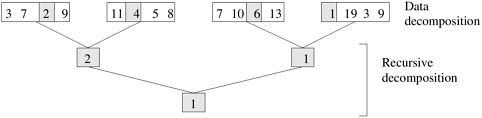
The problem of simulating a sequence of input jobs on the network described in Example 3.8 appears inherently sequential because the input of a typical component is the output of another. However, we can define speculative tasks that start simulating a subpart of the network, each assuming one of several possible inputs to that stage. When an actual input to a certain stage becomes available (as a result of the completion of another selector task from a previous stage), then all or part of the work required to simulate this input would have already been finished if the speculation was correct, or the simulation of this stage is restarted with the most recent correct input if the speculation was incorrect.

Speculative decomposition is different from exploratory decomposition in the following way. In speculative decomposition, the input at a branch leading to multiple parallel tasks is unknown, whereas in exploratory decomposition, the output of the multiple tasks originating at a branch is unknown. In speculative decomposition, the serial algorithm would strictly perform only one of the tasks at a speculative stage because when it reaches the beginning of that stage, it knows exactly which branch to take. Therefore, by preemptively computing for multiple possibilities out of which only one materializes, a parallel program employing speculative decomposition performs more aggregate work than its serial counterpart. Even if only one of the possibilities is explored speculatively, the parallel algorithm may perform more or the same amount of work as the serial algorithm. On the other hand, in exploratory decomposition, the serial algorithm too may explore different alternatives one after the other, because the branch that may lead to the solution is not known beforehand. Therefore, the parallel program may perform more, less, or the same amount of aggregate work compared to the serial algorithm depending on the location of the solution in the search space.

3.2.5 Hybrid Decompositions

So far we have discussed a number of decomposition methods that can be used to derive concurrent formulations of many algorithms. These decomposition techniques are not exclusive, and can often be combined together. Often, a computation is structured into multiple stages and it is sometimes necessary to apply different types of decomposition in different stages. For example, while finding the minimum of a large set of n numbers, a purely recursive decomposition may result in far more tasks than the number of processes, P, available. An efficient decomposition would partition the input into P roughly equal parts and have each task compute the minimum of the sequence assigned to it. The final result can be obtained by finding the minimum of the P intermediate results by using the recursive decomposition shown in Figure 3.21.

As another example of an application of hybrid decomposition, consider performing quicksort in parallel. In Example 3.4, we used a recursive decomposition to derive a concurrent formulation of quicksort. This formulation results in O(n) tasks for the problem of sorting a sequence of size n. But due to the dependencies among these tasks and due to uneven sizes of the tasks, the effective concurrency is quite limited. For example, the first task for splitting the input list into two parts takes O(n) time, which puts an upper limit on the performance gain possible via parallelization. But the step of splitting lists performed by tasks in parallel quicksort can also be decomposed using the input decomposition technique discussed in Section 9.4.1. The resulting hybrid decomposition that combines recursive decomposition and the input data-decomposition leads to a highly concurrent formulation of quicksort.