|
|
12.1 Overview of Dynamic ProgrammingWe start our discussion with a simple DP algorithm for computing shortest paths in a graph. Example 12.1 The shortest-path problem Consider a DP formulation for the problem of finding a shortest (least-cost) path between a pair of vertices in an acyclic graph. (Refer to Section 10.1 for an introduction to graph terminology.) An edge connecting node i to node j has cost c(i, j). If two vertices i and j are not connected then c(i, j) =
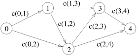
As an instance of this algorithm, consider the five-node acyclic graph shown in Figure 12.1. The problem is to find f (4). It can be computed given f (3) and f (2). More precisely,
Figure 12.1. A graph for which the shortest path between nodes 0 and 4 is to be computed.
Therefore, f (2) and f (3) are elements of the set of subproblems on which f (4) depends. Similarly, f (3) depends on f (1) and f (2),and f (1) and f (2) depend on f (0). Since f (0) is known, it is used to solve f (1) and f (2), which are used to solve f (3). In general, the solution to a DP problem is expressed as a minimum (or maximum) of possible alternate solutions. Each of these alternate solutions is constructed by composing one or more subproblems. If r represents the cost of a solution composed of subproblems x1, x2, ..., xl, then r can be written as
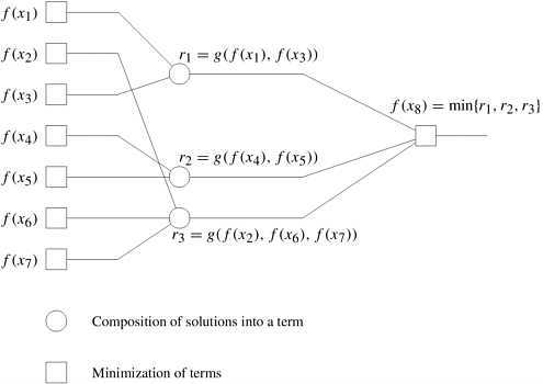
The function g is called the composition function, and its nature depends on the problem. If the optimal solution to each problem is determined by composing optimal solutions to the subproblems and selecting the minimum (or maximum), the formulation is said to be a DP formulation. Figure 12.2 illustrates an instance of composition and minimization of solutions. The solution to problem x8 is the minimum of the three possible solutions having costs r1, r2, and r3. The cost of the first solution is determined by composing solutions to subproblems x1 and x3, the second solution by composing solutions to subproblems x4 and x5, and the third solution by composing solutions to subproblems x2, x6, and x7. Figure 12.2. The computation and composition of subproblem solutions to solve problem f (x8).
DP represents the solution to an optimization problem as a recursive equation whose left side is an unknown quantity and whose right side is a minimization (or maximization) expression. Such an equation is called a functional equation or an optimization equation. In Equation 12.1, the composition function g is given by f (j) + c(j, x). This function is additive, since it is the sum of two terms. In a general DP formulation, the cost function need not be additive. A functional equation that contains a single recursive term (for example, f (j)) yields a monadic DP formulation. For an arbitrary DP formulation, the cost function may contain multiple recursive terms. DP formulations whose cost function contains multiple recursive terms are called polyadic formulations. The dependencies between subproblems in a DP formulation can be represented by a directed graph. Each node in the graph represents a subproblem. A directed edge from node i to node j indicates that the solution to the subproblem represented by node i is used to compute the solution to the subproblem represented by node j. If the graph is acyclic, then the nodes of the graph can be organized into levels such that subproblems at a particular level depend only on subproblems at previous levels. In this case, the DP formulation can be categorized as follows. If subproblems at all levels depend only on the results at the immediately preceding levels, the formulation is called a serial DP formulation; otherwise, it is called a nonserial DP formulation. Based on the preceding classification criteria, we define four classes of DP formulations: serial monadic, serial polyadic, nonserial monadic, and nonserial polyadic. These classes, however, are not exhaustive; some DP formulations cannot be classified into any of these categories. Due to the wide variety of problems solved using DP, it is difficult to develop generic parallel algorithms for them. However, parallel formulations of the problems in each of the four DP categories have certain similarities. In this chapter, we discuss parallel DP formulations for sample problems in each class. These samples suggest parallel algorithms for other problems in the same class. Note, however, that not all DP problems can be parallelized as illustrated in these examples. |
|
|
 . The graph contains