13.1 The Serial Algorithm

Consider a sequence X = <X [0], X [1], ..., X [n - 1]> of length n. The discrete Fourier transform of the sequence X is the sequence Y = <Y [0], Y [1], ..., Y [n - 1]>, where

Equation 13.1

In Equation 13.1, w is the primitive nth root of unity in the complex plane; that is, , where e is the base of natural logarithms. More generally, the powers of w in the equation can be thought of as elements of the finite commutative ring of integers modulo n. The powers of w used in an FFT computation are also known as twiddle factors.

The computation of each Y [i] according to Equation 13.1 requires n complex multiplications. Therefore, the sequential complexity of computing the entire sequence Y of length n is Q(n²). The fast Fourier transform algorithm described below reduces this complexity to Q(n log n).

Assume that n is a power of two. The FFT algorithm is based on the following step that permits an n-point DFT computation to be split into two (n/2)-point DFT computations:

Equation 13.2

Let ; that is, is the primitive (n/2)th root of unity. Then, we can rewrite Equation 13.2 as follows:

Equation 13.3

In Equation 13.3, each of the two summations on the right-hand side is an (n/2)-point DFT computation. If n is a power of two, each of these DFT computations can be divided similarly into smaller computations in a recursive manner. This leads to the recursive FFT algorithm given in Algorithm 13.1. This FFT algorithm is called the radix-2 algorithm because at each level of recursion, the input sequence is split into two equal halves.

Algorithm 13.1 The recursive, one-dimensional, unordered, radix-2 FFT algorithm. Here .

1.   procedure R_FFT(X, Y, n, w) 
2.   if (n = 1) then Y[0] := X[0] else 
3.   begin 
4.      R_FFT(<X[0], X[2], ..., X[n - 2]>, <Q[0], Q[1], ..., Q[n/2]>, n/2, w2); 
5.      R_FFT(<X[1], X[3], ..., X[n - 1]>, <T[0], T[1], ..., T[n/2]>, n/2, w2); 
6.      for i := 0 to n - 1 do 
7.          Y[i] :=Q[i mod (n/2)] + wi T[i mod (n/2)]; 
8.   end R_FFT 

Figure 13.1 illustrates how the recursive algorithm works on an 8-point sequence. As the figure shows, the first set of computations corresponding to line 7 of Algorithm 13.1 takes place at the deepest level of recursion. At this level, the elements of the sequence whose indices differ by n/2 are used in the computation. In each subsequent level, the difference between the indices of the elements used together in a computation decreases by a factor of two. The figure also shows the powers of w used in each computation.

The size of the input sequence over which an FFT is computed recursively decreases by a factor of two at each level of recursion (lines 4 and 5 of Algorithm 13.1). Hence, the maximum number of levels of recursion is log n for an initial sequence of length n. At the mth level of recursion, 2^m FFTs of size n/2^m each are computed. Thus, the total number of arithmetic operations (line 7) at each level is Q(n) and the overall sequential complexity of Algorithm 13.1 is Q(n log n).

The serial FFT algorithm can also be cast in an iterative form. The parallel implementations of the iterative form are easier to illustrate. Therefore, before describing parallel FFT algorithms, we give the iterative form of the serial algorithm. An iterative FFT algorithm is derived by casting each level of recursion, starting with the deepest level, as an iteration. Algorithm 13.2 gives the classic iterative Cooley-Tukey algorithm for an n-point, one-dimensional, unordered, radix-2 FFT. The program performs log n iterations of the outer loop starting on line 5. The value of the loop index m in the iterative version of the algorithm corresponds to the (log n - m)th level of recursion in the recursive version (Figure 13.1). Just as in each level of recursion, each iteration performs n complex multiplications and additions.

Algorithm 13.2 has two main loops. The outer loop starting at line 5 is executed log n times for an n-point FFT, and the inner loop starting at line 8 is executed n times during each iteration of the outer loop. All operations of the inner loop are constant-time arithmetic operations. Thus, the sequential time complexity of the algorithm is Q(n log n). In every iteration of the outer loop, the sequence R is updated using the elements that were stored in the sequence S during the previous iteration. For the first iteration, the input sequence X serves as the initial sequence R. The updated sequence X from the final iteration is the desired Fourier transform and is copied to the output sequence Y.

Algorithm 13.2 The Cooley-Tukey algorithm for one-dimensional, unordered, radix-2 FFT. Here .

1.   procedure ITERATIVE_FFT(X, Y, n) 
2.   begin 
3.      r := log n; 
4.      for i := 0 to n - 1 do R[i] := X[i]; 
5.      for m := 0 to r - 1 do        /* Outer loop */ 
6.          begin 
7.             for i := 0 to n - 1 do S[i]:= R[i]; 
8.             for i := 0 to n - 1 do /* Inner loop */ 
9.                 begin 
     /* Let (b0b1 ··· br -1) be the binary representation of i */ 
10.                   j := (b0...bm-10bm+1···br -1); 
11.                   k := (b0...bm-11bm+1···br -1); 
12.                   
13.            endfor;   /* Inner loop */ 
14.     endfor;          /* Outer loop */ 
15.     for i := 0 to n - 1 do Y[i] := R[i]; 
16.  end ITERATIVE_FFT 

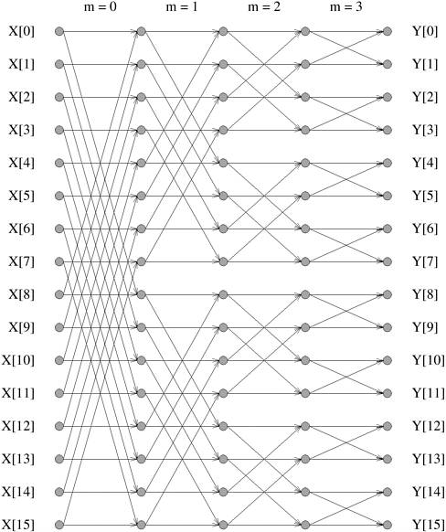
Line 12 in Algorithm 13.2 performs a crucial step in the FFT algorithm. This step updates R[i] by using S[j] and S[k]. The indices j and k are derived from the index i as follows. Assume that n = 2^r. Since0 i < n, the binary representation of i contains r bits. Let (b₀b₁ ···b_{r -1}) be the binary representation of index i. In the mth iteration of the outer loop (0 m < r), index j is derived by forcing the mth most significant bit of i (that is, b_m) to zero. Index k is derived by forcing b_m to 1. Thus, the binary representations of j and k differ only in their mth most significant bits. In the binary representation of i, b_m is either 0 or 1. Hence, of the two indices j and k, one is the same as index i, depending on whether b_m = 0 or b_m = 1. In the mth iteration of the outer loop, for each i between 0 and n - 1, R[i] is generated by executing line 12 of Algorithm 13.2 on S[i] and on another element of S whose index differs from i only in the mth most significant bit. Figure 13.2 shows the pattern in which these elements are paired for the case in which n = 16.