13.2 The Binary-Exchange Algorithm

This section discusses the binary-exchange algorithm for performing FFT on a parallel computer. First, a decomposition is induced by partitioning the input or the output vector. Therefore, each task starts with one element of the input vector and computes the corresponding element of the output. If each task is assigned the same label as the index of its input or output element, then in each of the log n iterations of the algorithm, exchange of data takes place between pairs of tasks with labels differing in one bit position.

13.2.1 A Full Bandwidth Network

In this subsection, we describe the implementation of the binary-exchange algorithm on a parallel computer on which a bisection width (Section 2.4.4) of Q(p) is available to p parallel processes. Since the pattern of interaction among the tasks of parallel FFT matches that of a hypercube network, we describe the algorithm assuming such an interconnection network. However, the performance and scalability analysis would be valid for any parallel computer with an overall simultaneous data-transfer capacity of O (p).

One Task Per Process

We first consider a simple mapping in which one task is assigned to each process. Figure 13.3 illustrates the interaction pattern induced by this mapping of the binary-exchange algorithm for n = 16. As the figure shows, process i (0 i < n) initially stores X [i] and finally generates Y [i]. In each of the log n iterations of the outer loop, process P_i updates the value of R[i] by executing line 12 of Algorithm 13.2. All n updates are performed in parallel.

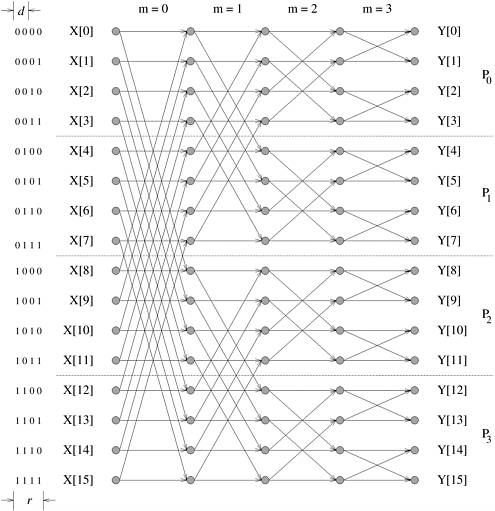
To perform the updates, process P_i requires an element of S from a process whose label differs from i at only one bit. Recall that in a hypercube, a node is connected to all those nodes whose labels differ from its own at only one bit position. Thus, the parallel FFT computation maps naturally onto a hypercube with a one-to-one mapping of processes to nodes. In the first iteration of the outer loop, the labels of each pair of communicating processes differ only at their most significant bits. For instance, processes P₀ to P₇ communicate with P₈ to P₁₅, respectively. Similarly, in the second iteration, the labels of processes communicating with each other differ at the second most significant bit, and so on.

In each of the log n iterations of this algorithm, every process performs one complex multiplication and addition, and exchanges one complex number with another process. Thus, there is a constant amount of work per iteration. Hence, it takes time Q(log n) to execute the algorithm in parallel by using a hypercube with n nodes. This hypercube formulation of FFT is cost-optimal because its process-time product is Q(n log n), the same as the complexity of a serial n-point FFT.

Multiple Tasks Per Process

We now consider a mapping in which the n tasks of an n-point FFT are mapped onto p processes, where n > p. For the sake of simplicity, let us assume that both n and p are powers of two, i.e., n = 2^r and p = 2^d. As Figure 13.4 shows, we partition the sequences into blocks of n/p contiguous elements and assign one block to each process.

An interesting property of the mapping shown in Figure 13.4 is that, if (b₀b₁ ··· b_{r -1}) is the binary representation of any i, such that 0 i < n, then R[i] and S[i] are mapped onto the process labeled (b₀···b_d-1). That is, the d most significant bits of the index of any element of the sequence are the binary representation of the label of the process that the element belongs to. This property of the mapping plays an important role in determining the amount of communication performed during the parallel execution of the FFT algorithm.

Figure 13.4 shows that elements with indices differing at their d (= 2) most significant bits are mapped onto different processes. However, all elements with indices having the same d most significant bits are mapped onto the same process. Recall from the previous section that an n-point FFT requires r = log n iterations of the outer loop. In the mth iteration of the loop, elements with indices differing in the mth most significant bit are combined. As a result, elements combined during the first d iterations belong to different processes, and pairs of elements combined during the last (r - d) iterations belong to the same processes. Hence, this parallel FFT algorithm requires interprocess interaction only during the first d = log p of the log n iterations. There is no interaction during the last r - d iterations. Furthermore, in the i th of the first d iterations, all the elements that a process requires come from exactly one other process - the one whose label is different at the i th most significant bit.

Each interaction operation exchanges n/p words of data. Therefore, the time spent in communication in the entire algorithm is t_s log p + t_w(n/p) log p. A process updates n/p elements of R during each of the log n iterations. If a complex multiplication and addition pair takes time t_c, then the parallel run time of the binary-exchange algorithm for n-point FFT on a p-node hypercube network is

Equation 13.4

The process-time product is t_cn log n + t_s p log p + t_wn log p. For the parallel system to be cost-optimal, this product should be O (n log n) - the sequential time complexity of the FFT algorithm. This is true for p n.

The expressions for speedup and efficiency are given by the following equations:

Equation 13.5

Scalability Analysis

From Section 13.1, we know that the problem size W for an n-point FFT is

Equation 13.6

Since an n-point FFT can utilize a maximum of n processes with the mapping of Figure 13.3, n p or n log n p log p to keep p processes busy. Thus, the isoefficiency function of this parallel FFT algorithm is W(p log p) due to concurrency. We now derive the isoefficiency function for the binary exchange algorithm due to the different communication-related terms. We can rewrite Equation 13.5 as

In order to maintain a fixed efficiency E , the expression (t_s p log p)/(t_cn log n) + (t_wlog p)/(t_c log n) should be equal to a constant 1/K, where K = E/(1 - E). We have defined the constant K in this manner to keep the terminology consistent with Chapter 5. As proposed in Section 5.4.2, we use an approximation to obtain closed expressions for the isoefficiency function. We first determine the rate of growth of the problem size with respect to p that would keep the terms due to t_s constant. To do this, we assume t_w = 0. Now the condition for maintaining constant efficiency E is as follows:

Equation 13.7

Equation 13.7 gives the isoefficiency function due to the overhead resulting from interaction latency or the message startup time.

Similarly, we derive the isoefficiency function due to the overhead resulting from t_w. We assume that t_s = 0; hence, a fixed efficiency E requires that the following relation be maintained:

Equation 13.8

If the term Kt_w/t_c is less than one, then the rate of growth of the problem size required by Equation 13.8 is less than Q(p log p). In this case, Equation 13.7 determines the overall isoefficiency function of this parallel system. However, if Kt_w/t_c exceeds one, then Equation 13.8 determines the overall isoefficiency function, which is now greater than the isoefficiency function of Q(p log p) given by Equation 13.7.

For this algorithm, the asymptotic isoefficiency function depends on the relative values of K, t_w, and t_c. Here, K is an increasing function of the efficiency E to be maintained, t_w depends on the communication bandwidth of the parallel computer, and t_c depends on the speed of the computation speed of the processors. The FFT algorithm is unique in that the order of the isoefficiency function depends on the desired efficiency and hardware-dependent parameters. In fact, the efficiency corresponding to Kt_w/t_c = 1(i.e.,1/(1 - E) = t_c/t_w, or E = t_c/(t_c + t_w)) acts as a kind of threshold. For a fixed t_c and t_w, efficiencies up to the threshold can be obtained easily. For E t_c/(t_c + t_w), the asymptotic isoefficiency function is Q(p log p). Efficiencies much higher than the threshold tc/(tc + t_w) can be obtained only if the problem size is extremely large. The reason is that for these efficiencies, the asymptotic isoefficiency function is Q. The following examples illustrate the effect of the value of Kt_w/t_c on the isoefficiency function.

Example 13.1 shows that there is a limit on the efficiency that can be obtained for reasonable problem sizes, and that the limit is determined by the ratio between the CPU speed and the communication bandwidth of the parallel computer being used. This limit can be raised by increasing the bandwidth of the communication channels. However, making the CPUs faster without increasing the communication bandwidth lowers the limit. Hence, the binary-exchange algorithm performs poorly on a parallel computer whose communication and computation speeds are not balanced. If the hardware is balanced with respect to its communication and computation speeds, then the binary-exchange algorithm is fairly scalable, and reasonable efficiencies can be maintained while increasing the problem size at the rate of Q(p log p).

13.2.2 Limited Bandwidth Network

Now we consider the implementation of the binary-exchange algorithm on a parallel computer whose cross-section bandwidth is less than Q(p). We choose a mesh interconnection network to illustrate the algorithm and its performance characteristics. Assume that n tasks are mapped onto p processes running on a mesh with rows and columns, and that is a power of two. Let n = 2^r and p = 2^d. Also assume that the processes are labeled in a row-major fashion and that the data are distributed in the same manner as for the hypercube; that is, an element with index (b₀b₁···b_{r -1}) is mapped onto the process labeled (b₀ ··· b_d-1).

As in case of the hypercube, communication takes place only during the first log p iterations between processes whose labels differ at one bit. However, unlike the hypercube, the communicating processes are not directly linked in a mesh. Consequently, messages travel over multiple links and there is overlap among messages sharing the same links. Figure 13.7 shows the messages sent and received by processes 0 and 37 during an FFT computation on a 64-node mesh. As the figure shows, process 0 communicates with processes 1, 2, 4, 8, 16, and 32. Note that all these processes lie in the same row or column of the mesh as that of process 0. Processes 1, 2, and 4 lie in the same row as process 0 at distances of 1, 2, and 4 links, respectively. Processes 8, 16, and 32 lie in the same column, again at distances of 1, 2, and 4 links. More precisely, in log of the log p steps that require communication, the communicating processes are in the same row, and in the remaining log steps, they are in the same column. The number of messages that share at least one link is equal to the number of links that each message traverses (Problem 13.9) because, during a given FFT iteration, all pairs of nodes exchange messages that traverse the same number of links.

The distance between the communicating processes in a row or a column grows from one link to links, doubling in each of the log iterations. This is true for any process in the mesh, such as process 37 shown in Figure 13.7. Thus, the total time spent in performing rowwise communication is . An equal amount of time is spent in columnwise communication. Recall that we assumed that a complex multiplication and addition pair takes time t_c. Since a process performs n/p such calculations in each of the log n iterations, the overall parallel run time is given by the following equation:

Equation 13.9

The speedup and efficiency are given by the following equations:

Equation 13.10

The process-time product of this parallel system is . The process-time product should be O (n log n) for cost-optimality, which is obtained when , or p = O (log² n). Since the communication term due to t_s in Equation 13.9 is the same as for the hypercube, the corresponding isoefficiency function is again Q(p log p) as given by Equation 13.7. By performing isoefficiency analysis along the same lines as in Section 13.2.1, we can show that the isoefficiency function due to the t_w term is (Problem 13.4). Given this isoefficiency function, the problem size must grow exponentially with the number of processes to maintain constant efficiency. Hence, the binary-exchange FFT algorithm is not very scalable on a mesh.

The communication overhead of the binary-exchange algorithm on a mesh cannot be reduced by using a different mapping of the sequences onto the processes. In any mapping, there is at least one iteration in which pairs of processes that communicate with each other are at least links apart (Problem 13.2). The algorithm inherently requires Q(p) bisection bandwidth on a p-node ensemble, and on an architecture like a 2-D mesh with Q bisection bandwidth, the communication time cannot be asymptotically better than as discussed above.

13.2.3 Extra Computations in Parallel FFT

So far, we have described a parallel formulation of the FFT algorithm on a hypercube and a mesh, and have discussed its performance and scalability in the presence of communication overhead on both architectures. In this section, we discuss another source of overhead that can be present in a parallel FFT implementation.

Recall from Algorithm 13.2 that the computation step of line 12 multiplies a power of w (a twiddle factor) with an element of S. For an n-point FFT, line 12 executes n log n times in the sequential algorithm. However, only n distinct powers of w (that is, w⁰, w¹, w², ..., w^n-1) are used in the entire algorithm. So some of the twiddle factors are used repeatedly. In a serial implementation, it is useful to precompute and store all n twiddle factors before starting the main algorithm. That way, the computation of twiddle factors requires only Q(n) complex operations rather than the Q(n log n) operations needed to compute all twiddle factors in each iteration of line 12.

In a parallel implementation, the total work required to compute the twiddle factors cannot be reduced to Q(n). The reason is that, even if a certain twiddle factor is used more than once, it might be used on different processes at different times. If FFTs of the same size are computed on the same number of processes, every process needs the same set of twiddle factors for each computation. In this case, the twiddle factors can be precomputed and stored, and the cost of their computation can be amortized over the execution of all instances of FFTs of the same size. However, if we consider only one instance of FFT, then twiddle factor computation gives rise to additional overhead in a parallel implementation, because it performs more overall operations than the sequential implementation.

As an example, consider the various powers of w used in the three iterations of an 8-point FFT. In the mth iteration of the loop starting on line 5 of the algorithm, w^l is computed for all i (0 i < n), such that l is the integer obtained by reversing the order of the m + 1 most significant bits of i and then padding them by log n - (m + 1) zeros to the right (refer to Figure 13.1 and Algorithm 13.2 to see how l is derived). Table 13.1 shows the binary representation of the powers of w required for all values of i and m for an 8-point FFT.

If eight processes are used, then each process computes and uses one column of Table 13.1. Process 0 computes just one twiddle factor for all its iterations, but some processes (in this case, all other processes 2-7) compute a new twiddle factor in each of the three iterations. If p = n/2 = 4, then each process computes two consecutive columns of the table. In this case, the last process computes the twiddle factors in the last two columns of the table. Hence, the last process computes a total of four different powers - one each for m = 0 (100) and m = 1 (110), and two for m = 2 (011 and 111). Although different processes may compute a different number of twiddle factors, the total overhead due to the extra work is proportional to p times the maximum number of twiddle factors that any single process computes. Let h(n, p) be the maximum number of twiddle factors that any of the p processes computes during an n-point FFT. Table 13.2 shows the values of h(8, p) for p = 1, 2, 4, and 8. The table also shows the maximum number of new twiddle factors that any single process computes in each iteration.

Table 13.1. The binary representation of the various powers of w calculated in different iterations of an 8-point FFT (also see Figure 13.1). The value of m refers to the iteration number of the outer loop, and i is the index of the inner loop of Algorithm 13.2.

	i
	0	1	2	3	4	5	6	7
m = 0	000	000	000	000	100	100	100	100
m = 1	000	000	100	100	010	010	110	110
m = 2	000	100	010	110	001	101	011	111

Table 13.2. The maximum number of new powers of w used by any process in each iteration of an 8-point FFT computation.

	p = 1	p = 2	p = 4	p = 8
m = 0	2	1	1	1
m = 1	2	2	1	1
m = 2	4	4	2	1
Total = h(8, p)	8	7	4	3

The function h is defined by the following recurrence relation (Problem 13.5):

The solution to this recurrence relation for p > 1 and n p is

Thus, if it takes time to compute one twiddle factor, then at least one process spends time log p computing twiddle factors. The total cost of twiddle factor computation, summed over all processes, is log p. Since even a serial implementation incurs a cost of in computing twiddle factors, the total parallel overhead due to extra work () is given by the following equation:

This overhead is independent of the architecture of the parallel computer used for the FFT computation. The isoefficiency function due to is Q(p log p). Since this term is of the same order as the isoefficiency terms due to message startup time and concurrency, the extra computations do not affect the overall scalability of parallel FFT.