3.4 Mapping Techniques for Load Balancing

Once a computation has been decomposed into tasks, these tasks are mapped onto processes with the objective that all tasks complete in the shortest amount of elapsed time. In order to achieve a small execution time, the overheads of executing the tasks in parallel must be minimized. For a given decomposition, there are two key sources of overhead. The time spent in inter-process interaction is one source of overhead. Another important source of overhead is the time that some processes may spend being idle. Some processes can be idle even before the overall computation is finished for a variety of reasons. Uneven load distribution may cause some processes to finish earlier than others. At times, all the unfinished tasks mapped onto a process may be waiting for tasks mapped onto other processes to finish in order to satisfy the constraints imposed by the task-dependency graph. Both interaction and idling are often a function of mapping. Therefore, a good mapping of tasks onto processes must strive to achieve the twin objectives of (1) reducing the amount of time processes spend in interacting with each other, and (2) reducing the total amount of time some processes are idle while the others are engaged in performing some tasks.

These two objectives often conflict with each other. For example, the objective of minimizing the interactions can be easily achieved by assigning sets of tasks that need to interact with each other onto the same process. In most cases, such a mapping will result in a highly unbalanced workload among the processes. In fact, following this strategy to the limit will often map all tasks onto a single process. As a result, the processes with a lighter load will be idle when those with a heavier load are trying to finish their tasks. Similarly, to balance the load among processes, it may be necessary to assign tasks that interact heavily to different processes. Due to the conflicts between these objectives, finding a good mapping is a nontrivial problem.

In this section, we will discuss various schemes for mapping tasks onto processes with the primary view of balancing the task workload of processes and minimizing their idle time. Reducing inter-process interaction is the topic of Section 3.5. The reader should be aware that assigning a balanced aggregate load of tasks to each process is a necessary but not sufficient condition for reducing process idling. Recall that the tasks resulting from a decomposition are not all ready for execution at the same time. A task-dependency graph determines which tasks can execute in parallel and which must wait for some others to

finish at a given stage in the execution of a parallel algorithm. Therefore, it is possible in a certain parallel formulation that although all processes perform the same aggregate amount of work, at different times, only a fraction of the processes are active while the remainder contain tasks that must wait for other tasks to finish. Similarly, poor synchronization among interacting tasks can lead to idling if one of the tasks has to wait to send or receive data from another task. A good mapping must ensure that the computations and interactions among processes at each stage of the execution of the parallel algorithm are well balanced. Figure 3.23 shows two mappings of 12-task decomposition in which the last four tasks can be started only after the first eight are finished due to dependencies among tasks. As the figure shows, two mappings, each with an overall balanced workload, can result in different completion times.

Mapping techniques used in parallel algorithms can be broadly classified into two categories: static and dynamic. The parallel programming paradigm and the characteristics of tasks and the interactions among them determine whether a static or a dynamic mapping is more suitable.

• Static Mapping: Static mapping techniques distribute the tasks among processes prior to the execution of the algorithm. For statically generated tasks, either static or dynamic mapping can be used. The choice of a good mapping in this case depends on several factors, including the knowledge of task sizes, the size of data associated with tasks, the characteristics of inter-task interactions, and even the parallel programming paradigm. Even when task sizes are known, in general, the problem of obtaining an optimal mapping is an NP-complete problem for non-uniform tasks. However, for many practical cases, relatively inexpensive heuristics provide fairly acceptable approximate solutions to the optimal static mapping problem.

  Algorithms that make use of static mapping are in general easier to design and program.

• Dynamic Mapping: Dynamic mapping techniques distribute the work among processes during the execution of the algorithm. If tasks are generated dynamically, then they must be mapped dynamically too. If task sizes are unknown, then a static mapping can potentially lead to serious load-imbalances and dynamic mappings are usually more effective. If the amount of data associated with tasks is large relative to the computation, then a dynamic mapping may entail moving this data among processes. The cost of this data movement may outweigh some other advantages of dynamic mapping and may render a static mapping more suitable. However, in a shared-address-space paradigm, dynamic mapping may work well even with large data associated with tasks if the interaction is read-only. The reader should be aware that the shared-address-space programming paradigm does not automatically provide immunity against data-movement costs. If the underlying hardware is NUMA (Section 2.3.2), then the data may physically move from a distant memory. Even in a cc-UMA architecture, the data may have to move from one cache to another.

  Algorithms that require dynamic mapping are usually more complicated, particularly in the message-passing programming paradigm.

Having discussed the guidelines for choosing between static and dynamic mappings, we now describe various schemes of these two types of mappings in detail.

3.4.1 Schemes for Static Mapping

Static mapping is often, though not exclusively, used in conjunction with a decomposition based on data partitioning. Static mapping is also used for mapping certain problems that are expressed naturally by a static task-dependency graph. In the following subsections, we will discuss mapping schemes based on data partitioning and task partitioning.

Mappings Based on Data Partitioning

In this section, we will discuss mappings based on partitioning two of the most common ways of representing data in algorithms, namely, arrays and graphs. The data-partitioning actually induces a decomposition, but the partitioning or the decomposition is selected with the final mapping in mind.

Array Distribution Schemes In a decomposition based on partitioning data, the tasks are closely associated with portions of data by the owner-computes rule. Therefore, mapping the relevant data onto the processes is equivalent to mapping tasks onto processes. We now study some commonly used techniques of distributing arrays or matrices among processes.

Block Distributions

Block distributions are some of the simplest ways to distribute an array and assign uniform contiguous portions of the array to different processes. In these distributions, a d-dimensional array is distributed among the processes such that each process receives a contiguous block of array entries along a specified subset of array dimensions. Block distributions of arrays are particularly suitable when there is a locality of interaction, i.e., computation of an element of an array requires other nearby elements in the array.

For example, consider an n x n two-dimensional array A with n rows and n columns. We can now select one of these dimensions, e.g., the first dimension, and partition the array into p parts such that the kth part contains rows kn/p...(k + 1)n/p - 1, where 0 k < p. That is, each partition contains a block of n/p consecutive rows of A. Similarly, if we partition A along the second dimension, then each partition contains a block of n/p consecutive columns. These row- and column-wise array distributions are illustrated in Figure 3.24.

Similarly, instead of selecting a single dimension, we can select multiple dimensions to partition. For instance, in the case of array A we can select both dimensions and partition the matrix into blocks such that each block corresponds to a n/p₁ x n/p₂ section of the matrix, with p = p₁ x p₂ being the number of processes. Figure 3.25 illustrates two different two-dimensional distributions, on a 4 x 4 and 2x 8 process grid, respectively. In general, given a d-dimensional array, we can distribute it using up to a d-dimensional block distribution.

Using these block distributions we can load-balance a variety of parallel computations that operate on multi-dimensional arrays. For example, consider the n x n matrix multiplication C = A x B , as discussed in Section 3.2.2. One way of decomposing this computation is to partition the output matrix C . Since each entry of C requires the same amount of computation, we can balance the computations by using either a one- or two-dimensional block distribution to partition C uniformly among the p available processes. In the first case, each process will get a block of n/p rows (or columns) of C, whereas in the second case, each process will get a block of size . In either case, the process will be responsible for computing the entries of the partition of C assigned to it.

As the matrix-multiplication example illustrates, quite often we have the choice of mapping the computations using either a one- or a two-dimensional distribution (and even more choices in the case of higher dimensional arrays). In general, higher dimensional distributions allow us to use more processes. For example, in the case of matrix-matrix multiplication, a one-dimensional distribution will allow us to use up to n processes by assigning a single row of C to each process. On the other hand, a two-dimensional distribution will allow us to use up to n² processes by assigning a single element of C to each process.

In addition to allowing a higher degree of concurrency, higher dimensional distributions also sometimes help in reducing the amount of interactions among the different processes for many problems. Figure 3.26 illustrates this in the case of dense matrix-multiplication. With a one-dimensional partitioning along the rows, each process needs to access the corresponding n/p rows of matrix A and the entire matrix B, as shown in Figure 3.26(a) for process P₅. Thus the total amount of data that needs to be accessed is n²/p + n². However, with a two-dimensional distribution, each process needs to access rows of matrix A and columns of matrix B, as shown in Figure 3.26(b) for process P₅. In the two-dimensional case, the total amount of shared data that each process needs to access is , which is significantly smaller compared to O(n²) shared data in the one-dimensional case.

Cyclic and Block-Cyclic Distributions

If the amount of work differs for different elements of a matrix, a block distribution can potentially lead to load imbalances. A classic example of this phenomenon is LU factorization of a matrix, in which the amount of computation increases from the top left to the bottom right of the matrix.

1.   procedure COL_LU (A) 
2.   begin 
3.      for k := 1 to n do 
4.          for j := k to n do 
5.              A[j, k]:= A[j, k]/A[k, k]; 
6.          endfor; 
7.          for j := k + 1 to n do 
8.              for i := k + 1 to n do 
9.                  A[i, j] := A[i, j] - A[i, k] x A[k, j]; 
10.             endfor; 
11.         endfor; 
   /* 
After this iteration, column A[k + 1 : n, k] is logically the kth 
column of L and row A[k, k : n] is logically the kth row of U. 
   */ 
12.     endfor; 
13.  end COL_LU 

For each iteration of the outer loop k := 1 to n, the next nested loop in Algorithm 3.3 goes from k + 1 to n. In other words, the active part of the matrix, as shown in Figure 3.28, shrinks towards the bottom right corner of the matrix as the computation proceeds. Therefore, in a block distribution, the processes assigned to the beginning rows and columns (i.e., left rows and top columns) would perform far less work than those assigned to the later rows and columns. For example, consider the decomposition for LU factorization shown in Figure 3.27 with a 3 x 3 two-dimensional block partitioning of the matrix. If we map all tasks associated with a certain block onto a process in a 9-process ensemble, then a significant amount of idle time will result. First, computing different blocks of the matrix requires different amounts of work. This is illustrated in Figure 3.29. For example, computing the final value of A_1,1 (which is actually L_1,1 U_1,1) requires only one task - Task 1. On the other hand, computing the final value of A_3,3 requires three tasks - Task 9, Task 13, and Task 14. Secondly, the process working on a block may idle even when there are unfinished tasks associated with that block. This idling can occur if the constraints imposed by the task-dependency graph do not allow the remaining tasks on this process to proceed until one or more tasks mapped onto other processes are completed.

The block-cyclic distribution is a variation of the block distribution scheme that can be used to alleviate the load-imbalance and idling problems. A detailed description of LU factorization with block-cyclic mapping is covered in Chapter 8, where it is shown how a block-cyclic mapping leads to a substantially more balanced work distribution than in Figure 3.29. The central idea behind a block-cyclic distribution is to partition an array into many more blocks than the number of available processes. Then we assign the partitions (and the associated tasks) to processes in a round-robin manner so that each process gets several non-adjacent blocks. More precisely, in a one-dimensional block-cyclic distribution of a matrix among p processes, the rows (columns) of an n x n matrix are divided into ap groups of n/(ap) consecutive rows (columns), where 1 a n/p. Now, these blocks are distributed among the p processes in a wraparound fashion such that block b_i is assigned to process P_{i %p} ('%' is the modulo operator). This distribution assigns a blocks of the matrix to each process, but each subsequent block that gets assigned to the same process is p blocks away. We can obtain a two-dimensional block-cyclic distribution of an n x n array by partitioning it into square blocks of size and distributing them on a hypothetical array of processes in a wraparound fashion. Similarly, the block-cyclic distribution can be extended to arrays of higher dimensions. Figure 3.30 illustrates one- and two-dimensional block cyclic distributions of a two-dimensional array.

The reason why a block-cyclic distribution is able to significantly reduce the amount of idling is that all processes have a sampling of tasks from all parts of the matrix. As a result, even if different parts of the matrix require different amounts of work, the overall work on each process balances out. Also, since the tasks assigned to a process belong to different parts of the matrix, there is a good chance that at least some of them are ready for execution at any given time.

Note that if we increase a to its upper limit of n/p, then each block is a single row (column) of the matrix in a one-dimensional block-cyclic distribution and a single element of the matrix in a two-dimensional block-cyclic distribution. Such a distribution is known as a cyclic distribution. A cyclic distribution is an extreme case of a block-cyclic distribution and can result in an almost perfect load balance due to the extreme fine-grained underlying decomposition. However, since a process does not have any contiguous data to work on, the resulting lack of locality may result in serious performance penalties. Additionally, such a decomposition usually leads to a high degree of interaction relative to the amount computation in each task. The lower limit of 1 for the value of a results in maximum locality and interaction optimality, but the distribution degenerates to a block distribution. Therefore, an appropriate value of a must be used to strike a balance between interaction conservation and load balance.

As in the case of block-distributions, higher dimensional block-cyclic distributions are usually preferable as they tend to incur a lower volume of inter-task interaction.

Randomized Block Distributions

A block-cyclic distribution may not always be able to balance computations when the distribution of work has some special patterns. For example, consider the sparse matrix shown in Figure 3.31(a) in which the shaded areas correspond to regions containing nonzero elements. If this matrix is distributed using a two-dimensional block-cyclic distribution, as illustrated in Figure 3.31(b), then we will end up assigning more non-zero blocks to the diagonal processes P₀, P₅, P₁₀, and P₁₅ than on any other processes. In fact some processes, like P₁₂, will not get any work.

Randomized block distribution, a more general form of the block distribution, can be used in situations illustrated in Figure 3.31. Just like a block-cyclic distribution, load balance is sought by partitioning the array into many more blocks than the number of available processes. However, the blocks are uniformly and randomly distributed among the processes. A one-dimensional randomized block distribution can be achieved as follows. A vector V of length ap (which is equal to the number of blocks) is used and V[j] is set to j for 0 j < ap. Now, V is randomly permuted, and process P_i is assigned the blocks stored in V[ia...(i + 1)a - 1]. Figure 3.32 illustrates this for p = 4 and a = 3. A two-dimensional randomized block distribution of an n x n array can be computed similarly by randomly permuting two vectors of length each and using them to choose the row and column indices of the blocks to be assigned to each process. As illustrated in Figure 3.33, the random block distribution is more effective in load balancing the computations performed in Figure 3.31.

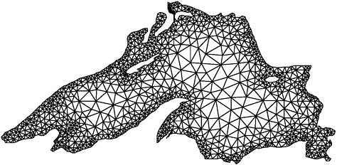
Graph Partitioning The array-based distribution schemes that we described so far are quite effective in balancing the computations and minimizing the interactions for a wide range of algorithms that use dense matrices and have structured and regular interaction patterns. However, there are many algorithms that operate on sparse data structures and for which the pattern of interaction among data elements is data dependent and highly irregular. Numerical simulations of physical phenomena provide a large source of such type of computations. In these computations, the physical domain is discretized and represented by a mesh of elements. The simulation of the physical phenomenon being modeled then involves computing the values of certain physical quantities at each mesh point. The computation at a mesh point usually requires data corresponding to that mesh point and to the points that are adjacent to it in the mesh. For example, Figure 3.34 shows a mesh imposed on Lake Superior. The simulation of a physical phenomenon such the dispersion of a water contaminant in the lake would now involve computing the level of contamination at each vertex of this mesh at various intervals of time.

Since, in general, the amount of computation at each point is the same, the load can be easily balanced by simply assigning the same number of mesh points to each process. However, if a distribution of the mesh points to processes does not strive to keep nearby mesh points together, then it may lead to high interaction overheads due to excessive data sharing. For example, if each process receives a random set of points as illustrated in Figure 3.35, then each process will need to access a large set of points belonging to other processes to complete computations for its assigned portion of the mesh.

Ideally, we would like to distribute the mesh points in a way that balances the load and at the same time minimizes the amount of data that each process needs to access in order to complete its computations. Therefore, we need to partition the mesh into p parts such that each part contains roughly the same number of mesh-points or vertices, and the number of edges that cross partition boundaries (i.e., those edges that connect points belonging to two different partitions) is minimized. Finding an exact optimal partition is an NP-complete problem. However, algorithms that employ powerful heuristics are available to compute reasonable partitions. After partitioning the mesh in this manner, each one of these p partitions is assigned to one of the p processes. As a result, each process is assigned a contiguous region of the mesh such that the total number of mesh points that needs to be accessed across partition boundaries is minimized. Figure 3.36 shows a good partitioning of the Lake Superior mesh - the kind that a typical graph partitioning software would generate.

Mappings Based on Task Partitioning

A mapping based on partitioning a task-dependency graph and mapping its nodes onto processes can be used when the computation is naturally expressible in the form of a static task-dependency graph with tasks of known sizes. As usual, this mapping must seek to achieve the often conflicting objectives of minimizing idle time and minimizing the interaction time of the parallel algorithm. Determining an optimal mapping for a general task-dependency graph is an NP-complete problem. However, specific situations often lend themselves to a simpler optimal or acceptable approximate solution.

As a simple example of a mapping based on task partitioning, consider a task-dependency graph that is a perfect binary tree. Such a task-dependency graph can occur in practical problems with recursive decomposition, such as the decomposition for finding the minimum of a list of numbers (Figure 3.9). Figure 3.37 shows a mapping of this task-dependency graph onto eight processes. It is easy to see that this mapping minimizes the interaction overhead by mapping many interdependent tasks onto the same process (i.e., the tasks along a straight branch of the tree) and others on processes only one communication link away from each other. Although there is some inevitable idling (e.g., when process 0 works on the root task, all other processes are idle), this idling is inherent in the task-dependency graph. The mapping shown in Figure 3.37 does not introduce any further idling and all tasks that are permitted to be concurrently active by the task-dependency graph are mapped onto different processes for parallel execution.

For some problems, an approximate solution to the problem of finding a good mapping can be obtained by partitioning the task-interaction graph. In the problem of modeling contaminant dispersion in Lake Superior discussed earlier in the context of data partitioning, we can define tasks such that each one of them is responsible for the computations associated with a certain mesh point. Now the mesh used to discretize the lake also acts as a task-interaction graph. Therefore, for this problem, using graph-partitioning to find a good mapping can also be viewed as task partitioning.

Another similar problem where task partitioning is applicable is that of sparse matrix-vector multiplication discussed in Section 3.1.2. A simple mapping of the task-interaction graph of Figure 3.6 is shown in Figure 3.38. This mapping assigns tasks corresponding to four consecutive entries of b to each process. Figure 3.39 shows another partitioning for the task-interaction graph of the sparse matrix vector multiplication problem shown in Figure 3.6 for three processes. The list Ci contains the indices of b that the tasks on Process i need to access from tasks mapped onto other processes. A quick comparison of the lists C0, C1, and C2 in the two cases readily reveals that the mapping based on partitioning the task interaction graph entails fewer exchanges of elements of b between processes than the naive mapping.

Hierarchical Mappings

Certain algorithms are naturally expressed as task-dependency graphs; however, a mapping based solely on the task-dependency graph may suffer from load-imbalance or inadequate concurrency. For example, in the binary-tree task-dependency graph of Figure 3.37, only a few tasks are available for concurrent execution in the top part of the tree. If the tasks are large enough, then a better mapping can be obtained by a further decomposition of the tasks into smaller subtasks. In the case where the task-dependency graph is a binary tree with four levels, the root task can be partitioned among eight processes, the tasks at the next level can be partitioned among four processes each, followed by tasks partitioned among two processes each at the next level. The eight leaf tasks can have a one-to-one mapping onto the processes. Figure 3.40 illustrates such a hierarchical mapping. Parallel quicksort introduced in Example 3.4 has a task-dependency graph similar to the one shown in Figure 3.37, and hence is an ideal candidate for a hierarchical mapping of the type shown in Figure 3.40.

An important practical problem to which the hierarchical mapping example discussed above applies directly is that of sparse matrix factorization. The high-level computations in sparse matrix factorization are guided by a task-dependency graph which is known as an elimination graph (elimination tree if the matrix is symmetric). However, the tasks in the elimination graph (especially the ones closer to the root) usually involve substantial computations and are further decomposed into subtasks using data-decomposition. A hierarchical mapping, using task partitioning at the top layer and array partitioning at the bottom layer, is then applied to this hybrid decomposition. In general, a hierarchical mapping can have many layers and different decomposition and mapping techniques may be suitable for different layers.

3.4.2 Schemes for Dynamic Mapping

Dynamic mapping is necessary in situations where a static mapping may result in a highly imbalanced distribution of work among processes or where the task-dependency graph itself if dynamic, thus precluding a static mapping. Since the primary reason for using a dynamic mapping is balancing the workload among processes, dynamic mapping is often referred to as dynamic load-balancing. Dynamic mapping techniques are usually classified as either centralized or distributed.

Centralized Schemes

In a centralized dynamic load balancing scheme, all executable tasks are maintained in a common central data structure or they are maintained by a special process or a subset of processes. If a special process is designated to manage the pool of available tasks, then it is often referred to as the master and the other processes that depend on the master to obtain work are referred to as slaves. Whenever a process has no work, it takes a portion of available work from the central data structure or the master process. Whenever a new task is generated, it is added to this centralized data structure or reported to the master process. Centralized load-balancing schemes are usually easier to implement than distributed schemes, but may have limited scalability. As more and more processes are used, the large number of accesses to the common data structure or the master process tends to become a bottleneck.

As an example of a scenario where centralized mapping may be applicable, consider the problem of sorting the entries in each row of an n x n matrix A. Serially, this can be accomplished by the following simple program segment:

1   for (i=1; i<n; i++) 
2     sort(A[i],n); 

Recall that the time to sort an array using some of the commonly used sorting algorithms, such as quicksort, can vary significantly depending on the initial order of the elements to be sorted. Therefore, each iteration of the loop in the program shown above can take different amounts of time. A naive mapping of the task of sorting an equal number of rows to each process may lead to load-imbalance. A possible solution to the potential load-imbalance problem in this case would be to maintain a central pool of indices of the rows that have yet to be sorted. Whenever a process is idle, it picks up an available index, deletes it, and sorts the row with that index, as long as the pool of indices is not empty. This method of scheduling the independent iterations of a loop among parallel processes is known as self scheduling.

The assignment of a single task to a process at a time is quite effective in balancing the computation; however, it may lead to bottlenecks in accessing the shared work queue, especially if each task (i.e., each loop iteration in this case) does not require a large enough amount of computation. If the average size of each task is M, and it takes D time to assign work to a process, then at most M/D processes can be kept busy effectively. The bottleneck can be eased by getting more than one task at a time. In chunk scheduling, every time a process runs out of work it gets a group of tasks. The potential problem with such a scheme is that it may lead to load-imbalances if the number of tasks (i.e., chunk) assigned in a single step is large. The danger of load-imbalance due to large chunk sizes can be reduced by decreasing the chunk-size as the program progresses. That is, initially the chunk size is large, but as the number of iterations left to be executed decreases, the chunk size also decreases. A variety of schemes have been developed for gradually adjusting the chunk size, that decrease the chunk size either linearly or non-linearly.

Distributed Schemes

In a distributed dynamic load balancing scheme, the set of executable tasks are distributed among processes which exchange tasks at run time to balance work. Each process can send work to or receive work from any other process. These methods do not suffer from the bottleneck associated with the centralized schemes. Some of the critical parameters of a distributed load balancing scheme are as follows:

• How are the sending and receiving processes paired together?

• Is the work transfer initiated by the sender or the receiver?

• How much work is transferred in each exchange? If too little work is transferred, then the receiver may not receive enough work and frequent transfers resulting in excessive interaction may be required. If too much work is transferred, then the sender may be out of work soon, again resulting in frequent transfers.

• When is the work transfer performed? For example, in receiver initiated load balancing, work may be requested when the process has actually run out of work or when the receiver has too little work left and anticipates being out of work soon.

A detailed study of each of these parameters is beyond the scope of this chapter. These load balancing schemes will be revisited in the context of parallel algorithms to which they apply when we discuss these algorithms in the later chapters - in particular, Chapter 11 in the context of parallel search algorithms.

Suitability to Parallel Architectures

Note that, in principle, both centralized and distributed mapping schemes can be implemented in both message-passing and shared-address-space paradigms. However, by its very nature any dynamic load balancing scheme requires movement of tasks from one process to another. Hence, for such schemes to be effective on message-passing computers, the size of the tasks in terms of computation should be much higher than the size of the data associated with the tasks. In a shared-address-space paradigm, the tasks don't need to be moved explicitly, although there is some implied movement of data to local caches or memory banks of processes. In general, the computational granularity of tasks to be moved can be much smaller on shared-address architecture than on message-passing architectures.