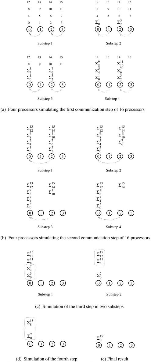
Example 5.7 illustrated an instance of an algorithm that is not cost-optimal. The algorithm discussed in this example uses as many processing elements as the number of inputs, which is excessive in terms of the number of processing elements. In practice, we assign larger pieces of input data to processing elements. This corresponds to increasing the granularity of computation on the processing elements. Using fewer than the maximum possible number of processing elements to execute a parallel algorithm is called scaling down a parallel system in terms of the number of processing elements. A naive way to scale down a parallel system is to design a parallel algorithm for one input element per processing element, and then use fewer processing elements to simulate a large number of processing elements. If there are n inputs and only p processing elements (p < n), we can use the parallel algorithm designed for n processing elements by assuming n virtual processing elements and having each of the p physical processing elements simulate n/p virtual processing elements.

As the number of processing elements decreases by a factor of n/p, the computation at each processing element increases by a factor of n/p because each processing element now performs the work of n/p processing elements. If virtual processing elements are mapped appropriately onto physical processing elements, the overall communication time does not grow by more than a factor of n/p. The total parallel runtime increases, at most, by a factor of n/p, and the processor-time product does not increase. Therefore, if a parallel system with n processing elements is cost-optimal, using p processing elements (where p < n)to simulate n processing elements preserves cost-optimality.

A drawback of this naive method of increasing computational granularity is that if a parallel system is not cost-optimal to begin with, it may still not be cost-optimal after the granularity of computation increases. This is illustrated by the following example for the problem of adding n numbers.

Example 5.9 Adding n numbers on p processing elements

Consider the problem of adding n numbers on p processing elements such that p < n and both n and p are powers of 2. We use the same algorithm as in Example 5.1 and simulate n processing elements on p processing elements. The steps leading to the solution are shown in Figure 5.5 for n = 16 and p = 4. Virtual processing element i is simulated by the physical processing element labeled i mod p; the numbers to be added are distributed similarly. The first log p of the log n steps of the original algorithm are simulated in (n/p) log p steps on p processing elements. In the remaining steps, no communication is required because the processing elements that communicate in the original algorithm are simulated by the same processing element; hence, the remaining numbers are added locally. The algorithm takes Q((n/p) log p) time in the steps that require communication, after which a single processing element is left with n/p numbers to add, taking time Q(n/p). Thus, the overall parallel execution time of this parallel system is Q((n/p) log p). Consequently, its cost is Q(n log p), which is asymptotically higher than the Q(n) cost of adding n numbers sequentially. Therefore, the parallel system is not cost-optimal.

Figure 5.5. Four processing elements simulating 16 processing elements to compute the sum of 16 numbers (first two steps). denotes the sum of numbers with consecutive labels from i to j . Four processing elements simulating 16 processing elements to compute the sum of 16 numbers (last three steps).

graphics/05fig13.jpg

Example 5.1 showed that n numbers can be added on an n-processor machine in time Q(log n). When using p processing elements to simulate n virtual processing elements (p < n), the expected parallel runtime is Q((n/p) log n). However, in Example 5.9 this task was performed in time Q((n/p) log p) instead. The reason is that every communication step of the original algorithm does not have to be simulated; at times, communication takes place between virtual processing elements that are simulated by the same physical processing element. For these operations, there is no associated overhead. For example, the simulation of the third and fourth steps (Figure 5.5(c) and (d)) did not require any communication. However, this reduction in communication was not enough to make the algorithm cost-optimal. Example 5.10 illustrates that the same problem (adding n numbers on p processing elements) can be performed cost-optimally with a smarter assignment of data to processing elements.

Example 5.10 Adding n numbers cost-optimally

An alternate method for adding n numbers using p processing elements is illustrated in Figure 5.6 for n = 16 and p = 4. In the first step of this algorithm, each processing element locally adds its n/p numbers in time Q(n/p). Now the problem is reduced to adding the p partial sums on p processing elements, which can be done in time Q(log p) by the method described in Example 5.1. The parallel runtime of this algorithm is

Equation 5.5

and its cost is Q(n + p log p). As long as n = W(p log p), the cost is Q(n), which is the same as the serial runtime. Hence, this parallel system is cost-optimal.

These simple examples demonstrate that the manner in which the computation is mapped onto processing elements may determine whether a parallel system is cost-optimal. Note, however, that we cannot make all non-cost-optimal systems cost-optimal by scaling down the number of processing elements.

5.3 The Effect of Granularity on Performance

Figure 5.5. Four processing elements simulating 16 processing elements to compute the sum of 16 numbers (first two steps). denotes the sum of numbers with consecutive labels from i to j . Four processing elements simulating 16 processing elements to compute the sum of 16 numbers (last three steps).

Figure 5.6. A cost-optimal way of computing the sum of 16 numbers using four processing elements.