5.2 Performance Metrics for Parallel Systems
It is important to study the performance of parallel programs with a view to determining the best algorithm, evaluating hardware platforms, and examining the benefits from parallelism. A number of metrics have been used based on the desired outcome of performance analysis.
5.2.1 Execution Time
The serial runtime of a program is the time elapsed between the beginning and the end of its execution on a sequential computer. The parallel runtime is the time that elapses from the moment a parallel computation starts to the moment the last processing element finishes execution. We denote the serial runtime by TS and the parallel runtime by TP.
5.2.2 Total Parallel Overhead
The overheads incurred by a parallel program are encapsulated into a single expression referred to as the overhead function. We define overhead function or total overhead of a parallel system as the total time collectively spent by all the processing elements over and above that required by the fastest known sequential algorithm for solving the same problem on a single processing element. We denote the overhead function of a parallel system by the symbol To.
The total time spent in solving a problem summed over all processing elements is pTP . TS units of this time are spent performing useful work, and the remainder is overhead. Therefore, the overhead function (To) is given by
Equation 5.1
5.2.3 Speedup
When evaluating a parallel system, we are often interested in knowing how much performance gain is achieved by parallelizing a given application over a sequential implementation. Speedup is a measure that captures the relative benefit of solving a problem in parallel. It is defined as the ratio of the time taken to solve a problem on a single processing element to the time required to solve the same problem on a parallel computer with p identical processing elements. We denote speedup by the symbol S.
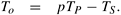
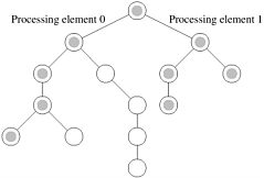
Example 5.1 Adding n numbers using n processing elements
Consider the problem of adding n numbers by using n processing elements. Initially, each processing element is assigned one of the numbers to be added and, at the end of the computation, one of the processing elements stores the sum of all the numbers. Assuming that n is a power of two, we can perform this operation in log n steps by propagating partial sums up a logical binary tree of processing elements. Figure 5.2 illustrates the procedure for n = 16. The processing elements are labeled from 0 to 15. Similarly, the 16 numbers to be added are labeled from 0 to 15. The sum of the numbers with consecutive labels from i to j is denoted by  . .
Each step shown in Figure 5.2 consists of one addition and the communication of a single word. The addition can be performed in some constant time, say tc, and the communication of a single word can be performed in time ts + tw. Therefore, the addition and communication operations take a constant amount of time. Thus,
Equation 5.2
Since the problem can be solved in Q(n) time on a single processing element, its speedup is
Equation 5.3

For a given problem, more than one sequential algorithm may be available, but all of these may not be equally suitable for parallelization. When a serial computer is used, it is natural to use the sequential algorithm that solves the problem in the least amount of time. Given a parallel algorithm, it is fair to judge its performance with respect to the fastest sequential algorithm for solving the same problem on a single processing element. Sometimes, the asymptotically fastest sequential algorithm to solve a problem is not known, or its runtime has a large constant that makes it impractical to implement. In such cases, we take the fastest known algorithm that would be a practical choice for a serial computer to be the best sequential algorithm. We compare the performance of a parallel algorithm to solve a problem with that of the best sequential algorithm to solve the same problem. We formally define the speedup S as the ratio of the serial runtime of the best sequential algorithm for solving a problem to the time taken by the parallel algorithm to solve the same problem on p processing elements. The p processing elements used by the parallel algorithm are assumed to be identical to the one used by the sequential algorithm.
Example 5.2 Computing speedups of parallel programs
Consider the example of parallelizing bubble sort (Section 9.3.1). Assume that a serial version of bubble sort of 105 records takes 150 seconds and a serial quicksort can sort the same list in 30 seconds. If a parallel version of bubble sort, also called odd-even sort, takes 40 seconds on four processing elements, it would appear that the parallel odd-even sort algorithm results in a speedup of 150/40 or 3.75. However, this conclusion is misleading, as in reality the parallel algorithm results in a speedup of 30/40 or 0.75 with respect to the best serial algorithm.
Theoretically, speedup can never exceed the number of processing elements, p. If the best sequential algorithm takes TS units of time to solve a given problem on a single processing element, then a speedup of p can be obtained on p processing elements if none of the processing elements spends more than time TS /p. A speedup greater than p is possible only if each processing element spends less than time TS /p solving the problem. In this case, a single processing element could emulate the p processing elements and solve the problem in fewer than TS units of time. This is a contradiction because speedup, by definition, is computed with respect to the best sequential algorithm. If TS is the serial runtime of the algorithm, then the problem cannot be solved in less than time TS on a single processing element.
In practice, a speedup greater than p is sometimes observed (a phenomenon known as superlinear speedup). This usually happens when the work performed by a serial algorithm is greater than its parallel formulation or due to hardware features that put the serial implementation at a disadvantage. For example, the data for a problem might be too large to fit into the cache of a single processing element, thereby degrading its performance due to the use of slower memory elements. But when partitioned among several processing elements, the individual data-partitions would be small enough to fit into their respective processing elements' caches. In the remainder of this book, we disregard superlinear speedup due to hierarchical memory.
Example 5.3 Superlinearity effects from caches
Consider the execution of a parallel program on a two-processor parallel system. The program attempts to solve a problem instance of size W. With this size and available cache of 64 KB on one processor, the program has a cache hit rate of 80%. Assuming the latency to cache of 2 ns and latency to DRAM of 100 ns, the effective memory access time is 2 x 0.8 + 100 x 0.2, or 21.6 ns. If the computation is memory bound and performs one FLOP/memory access, this corresponds to a processing rate of 46.3 MFLOPS. Now consider a situation when each of the two processors is effectively executing half of the problem instance (i.e., size W/2). At this problem size, the cache hit ratio is expected to be higher, since the effective problem size is smaller. Let us assume that the cache hit ratio is 90%, 8% of the remaining data comes from local DRAM, and the other 2% comes from the remote DRAM (communication overhead). Assuming that remote data access takes 400 ns, this corresponds to an overall access time of 2 x 0.9 + 100 x 0.08 + 400 x 0.02, or 17.8 ns. The corresponding execution rate at each processor is therefore 56.18, for a total execution rate of 112.36 MFLOPS. The speedup in this case is given by the increase in speed over serial formulation, i.e., 112.36/46.3 or 2.43! Here, because of increased cache hit ratio resulting from lower problem size per processor, we notice superlinear speedup.
Example 5.4 Superlinearity effects due to exploratory decomposition
Consider an algorithm for exploring leaf nodes of an unstructured tree. Each leaf has a label associated with it and the objective is to find a node with a specified label, in this case 'S'. Such computations are often used to solve combinatorial problems, where the label 'S' could imply the solution to the problem (Section 11.6). In Figure 5.3, we illustrate such a tree. The solution node is the rightmost leaf in the tree. A serial formulation of this problem based on depth-first tree traversal explores the entire tree, i.e., all 14 nodes. If it takes time tc to visit a node, the time for this traversal is 14tc. Now consider a parallel formulation in which the left subtree is explored by processing element 0 and the right subtree by processing element 1. If both processing elements explore the tree at the same speed, the parallel formulation explores only the shaded nodes before the solution is found. Notice that the total work done by the parallel algorithm is only nine node expansions, i.e., 9tc. The corresponding parallel time, assuming the root node expansion is serial, is 5tc (one root node expansion, followed by four node expansions by each processing element). The speedup of this two-processor execution is therefore 14tc/5tc , or 2.8!
The cause for this superlinearity is that the work performed by parallel and serial algorithms is different. Indeed, if the two-processor algorithm was implemented as two processes on the same processing element, the algorithmic superlinearity would disappear for this problem instance. Note that when exploratory decomposition is used, the relative amount of work performed by serial and parallel algorithms is dependent upon the location of the solution, and it is often not possible to find a serial algorithm that is optimal for all instances. Such effects are further analyzed in greater detail in Chapter 11.
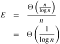
5.2.4 Efficiency
Only an ideal parallel system containing p processing elements can deliver a speedup equal to p. In practice, ideal behavior is not achieved because while executing a parallel algorithm, the processing elements cannot devote 100% of their time to the computations of the algorithm. As we saw in Example 5.1, part of the time required by the processing elements to compute the sum of n numbers is spent idling (and communicating in real systems). Efficiency is a measure of the fraction of time for which a processing element is usefully employed; it is defined as the ratio of speedup to the number of processing elements. In an ideal parallel system, speedup is equal to p and efficiency is equal to one. In practice, speedup is less than p and efficiency is between zero and one, depending on the effectiveness with which the processing elements are utilized. We denote efficiency by the symbol E. Mathematically, it is given by
Equation 5.4

Example 5.5 Efficiency of adding n numbers on n processing elements
From Equation 5.3 and the preceding definition, the efficiency of the algorithm for adding n numbers on n processing elements is
We also illustrate the process of deriving the parallel runtime, speedup, and efficiency while preserving various constants associated with the parallel platform.
Example 5.6 Edge detection on images
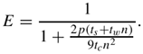
Given an n x n pixel image, the problem of detecting edges corresponds to applying a3x 3 template to each pixel. The process of applying the template corresponds to multiplying pixel values with corresponding template values and summing across the template (a convolution operation). This process is illustrated in Figure 5.4(a) along with typical templates (Figure 5.4(b)). Since we have nine multiply-add operations for each pixel, if each multiply-add takes time tc, the entire operation takes time 9tcn2 on a serial computer.
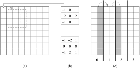
A simple parallel algorithm for this problem partitions the image equally across the processing elements and each processing element applies the template to its own subimage. Note that for applying the template to the boundary pixels, a processing element must get data that is assigned to the adjoining processing element. Specifically, if a processing element is assigned a vertically sliced subimage of dimension n x (n/p), it must access a single layer of n pixels from the processing element to the left and a single layer of n pixels from the processing element to the right (note that one of these accesses is redundant for the two processing elements assigned the subimages at the extremities). This is illustrated in Figure 5.4(c).
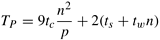
On a message passing machine, the algorithm executes in two steps: (i) exchange a layer of n pixels with each of the two adjoining processing elements; and (ii) apply template on local subimage. The first step involves two n-word messages (assuming each pixel takes a word to communicate RGB data). This takes time 2(ts + twn). The second step takes time 9tcn2/p. The total time for the algorithm is therefore given by:
The corresponding values of speedup and efficiency are given by:
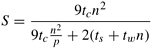
and
5.2.5 Cost
We define the cost of solving a problem on a parallel system as the product of parallel runtime and the number of processing elements used. Cost reflects the sum of the time that each processing element spends solving the problem. Efficiency can also be expressed as the ratio of the execution time of the fastest known sequential algorithm for solving a problem to the cost of solving the same problem on p processing elements.
The cost of solving a problem on a single processing element is the execution time of the fastest known sequential algorithm. A parallel system is said to be cost-optimal if the cost of solving a problem on a parallel computer has the same asymptotic growth (in Q terms) as a function of the input size as the fastest-known sequential algorithm on a single processing element. Since efficiency is the ratio of sequential cost to parallel cost, a cost-optimal parallel system has an efficiency of Q(1).
Cost is sometimes referred to as work or processor-time product, and a cost-optimal system is also known as a pTP -optimal system.
Example 5.7 Cost of adding n numbers on n processing elements
The algorithm given in Example 5.1 for adding n numbers on n processing elements has a processor-time product of Q(n log n). Since the serial runtime of this operation is Q(n), the algorithm is not cost optimal.
Cost optimality is a very important practical concept although it is defined in terms of asymptotics. We illustrate this using the following example.
Example 5.8 Performance of non-cost optimal algorithms
Consider a sorting algorithm that uses n processing elements to sort the list in time (log n)2. Since the serial runtime of a (comparison-based) sort is n log n, the speedup and efficiency of this algorithm are given by n/log n and 1/log n, respectively. The pTP product of this algorithm is n(log n)2. Therefore, this algorithm is not cost optimal but only by a factor of log n. Let us consider a realistic scenario in which the number of processing elements p is much less than n. An assignment of these n tasks to p < n processing elements gives us a parallel time less than n(log n)2/p. This follows from the fact that if n processing elements take time (log n)2, then one processing element would take time n(log n)2; and p processing elements would take time n(log n)2/p. The corresponding speedup of this formulation is p/log n. Consider the problem of sorting 1024 numbers (n = 1024, log n = 10) on 32 processing elements. The speedup expected is only p/log n or 3.2. This number gets worse as n increases. For n = 106, log n = 20 and the speedup is only 1.6. Clearly, there is a significant cost associated with not being cost-optimal even by a very small factor (note that a factor of log p is smaller than even  ). This emphasizes the practical importance of cost-optimality. ). This emphasizes the practical importance of cost-optimality.
|