|
|
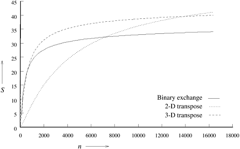
5.4 Scalability of Parallel SystemsVery often, programs are designed and tested for smaller problems on fewer processing elements. However, the real problems these programs are intended to solve are much larger, and the machines contain larger number of processing elements. Whereas code development is simplified by using scaled-down versions of the machine and the problem, their performance and correctness (of programs) is much more difficult to establish based on scaled-down systems. In this section, we will investigate techniques for evaluating the scalability of parallel programs using analytical tools. Example 5.11 Why is performance extrapolation so difficult? Consider three parallel algorithms for computing an n-point Fast Fourier Transform (FFT) on 64 processing elements. Figure 5.7 illustrates speedup as the value of n is increased to 18 K. Keeping the number of processing elements constant, at smaller values of n, one would infer from observed speedups that binary exchange and 3-D transpose algorithms are the best. However, as the problem is scaled up to 18 K points or more, it is evident from Figure 5.7 that the 2-D transpose algorithm yields best speedup. (These algorithms are discussed in greater detail in Chapter 13.) Figure 5.7. A comparison of the speedups obtained by the binary-exchange, 2-D transpose and 3-D transpose algorithms on 64 processing elements with tc = 2, tw = 4, ts = 25, and th = 2 (see Chapter 13 for details).
Similar results can be shown relating to the variation in number of processing elements as the problem size is held constant. Unfortunately, such parallel performance traces are the norm as opposed to the exception, making performance prediction based on limited observed data very difficult. 5.4.1 Scaling Characteristics of Parallel ProgramsThe efficiency of a parallel program can be written as:
Using the expression for parallel overhead (Equation 5.1), we can rewrite this expression as
The total overhead function To is an increasing function of p. This is because every program must contain some serial component. If this serial component of the program takes time tserial, then during this time all the other processing elements must be idle. This corresponds to a total overhead function of (p - 1) x tserial. Therefore, the total overhead function To grows at least linearly with p. In addition, due to communication, idling, and excess computation, this function may grow superlinearly in the number of processing elements. Equation 5.6 gives us several interesting insights into the scaling of parallel programs. First, for a given problem size (i.e. the value of TS remains constant), as we increase the number of processing elements, To increases. In such a scenario, it is clear from Equation 5.6 that the overall efficiency of the parallel program goes down. This characteristic of decreasing efficiency with increasing number of processing elements for a given problem size is common to all parallel programs. Example 5.12 Speedup and efficiency as functions of the number of processing elements Consider the problem of adding n numbers on p processing elements. We use the same algorithm as in Example 5.10. However, to illustrate actual speedups, we work with constants here instead of asymptotics. Assuming unit time for adding two numbers, the first phase (local summations) of the algorithm takes roughly n/p time. The second phase involves log p steps with a communication and an addition at each step. If a single communication takes unit time as well, the time for this phase is 2 log p. Therefore, we can derive parallel time, speedup, and efficiency as:
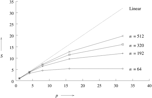
These expressions can be used to calculate the speedup and efficiency for any pair of n and p. Figure 5.8 shows the S versus p curves for a few different values of n and p. Table 5.1 shows the corresponding efficiencies. Figure 5.8. Speedup versus the number of processing elements for adding a list of numbers.
Figure 5.8 and Table 5.1 illustrate that the speedup tends to saturate and efficiency drops as a consequence of Amdahl's law (Problem 5.1). Furthermore, a larger instance of the same problem yields higher speedup and efficiency for the same number of processing elements, although both speedup and efficiency continue to drop with increasing p. Let us investigate the effect of increasing the problem size keeping the number of processing elements constant. We know that the total overhead function To is a function of both problem size TS and the number of processing elements p. In many cases, To grows sublinearly with respect to TS . In such cases, we can see that efficiency increases if the problem size is increased keeping the number of processing elements constant. For such algorithms, it should be possible to keep the efficiency fixed by increasing both the size of the problem and the number of processing elements simultaneously. For instance, in Table 5.1, the efficiency of adding 64 numbers using four processing elements is 0.80. If the number of processing elements is increased to 8 and the size of the problem is scaled up to add 192 numbers, the efficiency remains 0.80. Increasing p to 16 and n to 512 results in the same efficiency. This ability to maintain efficiency at a fixed value by simultaneously increasing the number of processing elements and the size of the problem is exhibited by many parallel systems. We call such systems scalable parallel systems. The scalability of a parallel system is a measure of its capacity to increase speedup in proportion to the number of processing elements. It reflects a parallel system's ability to utilize increasing processing resources effectively.
Recall from Section 5.2.5 that a cost-optimal parallel system has an efficiency of Q(1). Therefore, scalability and cost-optimality of parallel systems are related. A scalable parallel system can always be made cost-optimal if the number of processing elements and the size of the computation are chosen appropriately. For instance, Example 5.10 shows that the parallel system for adding n numbers on p processing elements is cost-optimal when n = W(p log p). Example 5.13 shows that the same parallel system is scalable if n is increased in proportion to Q(p log p) as p is increased. Example 5.13 Scalability of adding n numbers For the cost-optimal addition of n numbers on p processing elements n = W(p log p). As shown in Table 5.1, the efficiency is 0.80 for n = 64 and p = 4. At this point, the relation between n and p is n = 8 p log p. If the number of processing elements is increased to eight, then 8 p log p = 192. Table 5.1 shows that the efficiency is indeed 0.80 with n = 192 for eight processing elements. Similarly, for p = 16, the efficiency is 0.80 for n = 8 p log p = 512. Thus, this parallel system remains cost-optimal at an efficiency of 0.80 if n is increased as 8 p log p. 5.4.2 The Isoefficiency Metric of ScalabilityWe summarize the discussion in the section above with the following two observations:
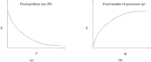
These two phenomena are illustrated in Figure 5.9(a) and (b), respectively. Following from these two observations, we define a scalable parallel system as one in which the efficiency can be kept constant as the number of processing elements is increased, provided that the problem size is also increased. It is useful to determine the rate at which the problem size must increase with respect to the number of processing elements to keep the efficiency fixed. For different parallel systems, the problem size must increase at different rates in order to maintain a fixed efficiency as the number of processing elements is increased. This rate determines the degree of scalability of the parallel system. As we shall show, a lower rate is more desirable than a higher growth rate in problem size. Let us now investigate metrics for quantitatively determining the degree of scalability of a parallel system. However, before we do that, we must define the notion of problem size precisely. Figure 5.9. Variation of efficiency: (a) as the number of processing elements is increased for a given problem size; and (b) as the problem size is increased for a given number of processing elements. The phenomenon illustrated in graph (b) is not common to all parallel systems.
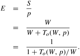
Problem Size When analyzing parallel systems, we frequently encounter the notion of the size of the problem being solved. Thus far, we have used the term problem size informally, without giving a precise definition. A naive way to express problem size is as a parameter of the input size; for instance, n in case of a matrix operation involving n x n matrices. A drawback of this definition is that the interpretation of problem size changes from one problem to another. For example, doubling the input size results in an eight-fold increase in the execution time for matrix multiplication and a four-fold increase for matrix addition (assuming that the conventional Q(n3) algorithm is the best matrix multiplication algorithm, and disregarding more complicated algorithms with better asymptotic complexities). A consistent definition of the size or the magnitude of the problem should be such that, regardless of the problem, doubling the problem size always means performing twice the amount of computation. Therefore, we choose to express problem size in terms of the total number of basic operations required to solve the problem. By this definition, the problem size is Q(n3) for n x n matrix multiplication (assuming the conventional algorithm) and Q(n2) for n x n matrix addition. In order to keep it unique for a given problem, we define problem size as the number of basic computation steps in the best sequential algorithm to solve the problem on a single processing element, where the best sequential algorithm is defined as in Section 5.2.3. Because it is defined in terms of sequential time complexity, the problem size is a function of the size of the input. The symbol we use to denote problem size is W. In the remainder of this chapter, we assume that it takes unit time to perform one basic computation step of an algorithm. This assumption does not impact the analysis of any parallel system because the other hardware-related constants, such as message startup time, per-word transfer time, and per-hop time, can be normalized with respect to the time taken by a basic computation step. With this assumption, the problem size W is equal to the serial runtime TS of the fastest known algorithm to solve the problem on a sequential computer. The Isoefficiency FunctionParallel execution time can be expressed as a function of problem size, overhead function, and the number of processing elements. We can write parallel runtime as:
The resulting expression for speedup is
Finally, we write the expression for efficiency as
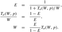
In Equation 5.12, if the problem size is kept constant and p is increased, the efficiency decreases because the total overhead To increases with p. If W is increased keeping the number of processing elements fixed, then for scalable parallel systems, the efficiency increases. This is because To grows slower than Q(W) for a fixed p. For these parallel systems, efficiency can be maintained at a desired value (between 0 and 1) for increasing p, provided W is also increased. For different parallel systems, W must be increased at different rates with respect to p in order to maintain a fixed efficiency. For instance, in some cases, W might need to grow as an exponential function of p to keep the efficiency from dropping as p increases. Such parallel systems are poorly scalable. The reason is that on these parallel systems it is difficult to obtain good speedups for a large number of processing elements unless the problem size is enormous. On the other hand, if W needs to grow only linearly with respect to p, then the parallel system is highly scalable. That is because it can easily deliver speedups proportional to the number of processing elements for reasonable problem sizes. For scalable parallel systems, efficiency can be maintained at a fixed value (between 0 and 1) if the ratio To/W in Equation 5.12 is maintained at a constant value. For a desired value E of efficiency,
Let K = E/(1 - E) be a constant depending on the efficiency to be maintained. Since To is a function of W and p, Equation 5.13 can be rewritten as
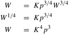
From Equation 5.14, the problem size W can usually be obtained as a function of p by algebraic manipulations. This function dictates the growth rate of W required to keep the efficiency fixed as p increases. We call this function the isoefficiency function of the parallel system. The isoefficiency function determines the ease with which a parallel system can maintain a constant efficiency and hence achieve speedups increasing in proportion to the number of processing elements. A small isoefficiency function means that small increments in the problem size are sufficient for the efficient utilization of an increasing number of processing elements, indicating that the parallel system is highly scalable. However, a large isoefficiency function indicates a poorly scalable parallel system. The isoefficiency function does not exist for unscalable parallel systems, because in such systems the efficiency cannot be kept at any constant value as p increases, no matter how fast the problem size is increased. Example 5.14 Isoefficiency function of adding numbers The overhead function for the problem of adding n numbers on p processing elements is approximately 2 p log p, as given by Equations 5.9 and 5.1. Substituting To by 2 p log p in Equation 5.14, we get
Thus, the asymptotic isoefficiency function for this parallel system is Q(p log p). This means that, if the number of processing elements is increased from p to p', the problem size (in this case, n) must be increased by a factor of (p' log p')/(p log p) to get the same efficiency as on p processing elements. In other words, increasing the number of processing elements by a factor of p'/p requires that n be increased by a factor of (p' log p')/(p log p) to increase the speedup by a factor of p'/p. In the simple example of adding n numbers, the overhead due to communication (hereafter referred to as the communication overhead) is a function of p only. In general, communication overhead can depend on both the problem size and the number of processing elements. A typical overhead function can have several distinct terms of different orders of magnitude with respect to p and W. In such a case, it can be cumbersome (or even impossible) to obtain the isoefficiency function as a closed function of p. For example, consider a hypothetical parallel system for which To = p3/2 + p3/4 W 3/4. For this overhead function, Equation 5.14 can be rewritten as W = Kp3/2 + Kp3/4 W 3/4. It is hard to solve this equation for W in terms of p. Recall that the condition for constant efficiency is that the ratio To/W remains fixed. As p and W increase, the efficiency is nondecreasing as long as none of the terms of To grow faster than W. If To has multiple terms, we balance W against each term of To and compute the respective isoefficiency functions for individual terms. The component of To that requires the problem size to grow at the highest rate with respect to p determines the overall asymptotic isoefficiency function of the parallel system. Example 5.15 further illustrates this technique of isoefficiency analysis. Example 5.15 Isoefficiency function of a parallel system with a complex overhead function Consider a parallel system for which To = p3/2 + p3/4 W 3/4. Using only the first term of To in Equation 5.14, we get
Using only the second term, Equation 5.14 yields the following relation between W and p:
To ensure that the efficiency does not decrease as the number of processing elements increases, the first and second terms of the overhead function require the problem size to grow as Q(p3/2) and Q(p3), respectively. The asymptotically higher of the two rates, Q(p3), gives the overall asymptotic isoefficiency function of this parallel system, since it subsumes the rate dictated by the other term. The reader may indeed verify that if the problem size is increased at this rate, the efficiency is Q(1) and that any rate lower than this causes the efficiency to fall with increasing p. In a single expression, the isoefficiency function captures the characteristics of a parallel algorithm as well as the parallel architecture on which it is implemented. After performing isoefficiency analysis, we can test the performance of a parallel program on a few processing elements and then predict its performance on a larger number of processing elements. However, the utility of isoefficiency analysis is not limited to predicting the impact on performance of an increasing number of processing elements. Section 5.4.5 shows how the isoefficiency function characterizes the amount of parallelism inherent in a parallel algorithm. We will see in Chapter 13 that isoefficiency analysis can also be used to study the behavior of a parallel system with respect to changes in hardware parameters such as the speed of processing elements and communication channels. Chapter 11 illustrates how isoefficiency analysis can be used even for parallel algorithms for which we cannot derive a value of parallel runtime. 5.4.3 Cost-Optimality and the Isoefficiency FunctionIn Section 5.2.5, we stated that a parallel system is cost-optimal if the product of the number of processing elements and the parallel execution time is proportional to the execution time of the fastest known sequential algorithm on a single processing element. In other words, a parallel system is cost-optimal if and only if
Substituting the expression for TP from the right-hand side of Equation 5.10, we get the following:
Equations 5.19 and 5.20 suggest that a parallel system is cost-optimal if and only if its overhead function does not asymptotically exceed the problem size. This is very similar to the condition given by Equation 5.14 for maintaining a fixed efficiency while increasing the number of processing elements in a parallel system. If Equation 5.14 yields an isoefficiency function f(p), then it follows from Equation 5.20 that the relation W = W(f(p)) must be satisfied to ensure the cost-optimality of a parallel system as it is scaled up. The following example further illustrates the relationship between cost-optimality and the isoefficiency function. Example 5.16 Relationship between cost-optimality and isoefficiency Consider the cost-optimal solution to the problem of adding n numbers on p processing elements, presented in Example 5.10. For this parallel system, W 5.4.4 A Lower Bound on the Isoefficiency FunctionWe discussed earlier that a smaller isoefficiency function indicates higher scalability. Accordingly, an ideally-scalable parallel system must have the lowest possible isoefficiency function. For a problem consisting of W units of work, no more than W processing elements can be used cost-optimally; additional processing elements will be idle. If the problem size grows at a rate slower than Q(p) as the number of processing elements increases, then the number of processing elements will eventually exceed W. Even for an ideal parallel system with no communication, or other overhead, the efficiency will drop because processing elements added beyond p = W will be idle. Thus, asymptotically, the problem size must increase at least as fast as Q(p) to maintain fixed efficiency; hence, W(p) is the asymptotic lower bound on the isoefficiency function. It follows that the isoefficiency function of an ideally scalable parallel system is Q(p). 5.4.5 The Degree of Concurrency and the Isoefficiency FunctionA lower bound of W(p) is imposed on the isoefficiency function of a parallel system by the number of operations that can be performed concurrently. The maximum number of tasks that can be executed simultaneously at any time in a parallel algorithm is called its degree of concurrency. The degree of concurrency is a measure of the number of operations that an algorithm can perform in parallel for a problem of size W; it is independent of the parallel architecture. If C(W) is the degree of concurrency of a parallel algorithm, then for a problem of size W, no more than C(W) processing elements can be employed effectively. Example 5.17 Effect of concurrency on isoefficiency function Consider solving a system of n equations in n variables by using Gaussian elimination (Section 8.3.1). The total amount of computation is Q(n3). But then variables must be eliminated one after the other, and eliminating each variable requires Q(n2) computations. Thus, at most Q(n2) processing elements can be kept busy at any time. Since W = Q(n3) for this problem, the degree of concurrency C(W) is Q(W2/3) and at most Q(W2/3) processing elements can be used efficiently. On the other hand, given p processing elements, the problem size should be at least W(p3/2) to use them all. Thus, the isoefficiency function of this computation due to concurrency is Q(p3/2). The isoefficiency function due to concurrency is optimal (that is, Q(p)) only if the degree of concurrency of the parallel algorithm is Q(W). If the degree of concurrency of an algorithm is less than Q(W), then the isoefficiency function due to concurrency is worse (that is, greater) than Q(p). In such cases, the overall isoefficiency function of a parallel system is given by the maximum of the isoefficiency functions due to concurrency, communication, and other overheads. |
|
|