8.2 Matrix-Matrix Multiplication

This section discusses parallel algorithms for multiplying two n x n dense, square matrices A and B to yield the product matrix C = A x B. All parallel matrix multiplication algorithms in this chapter are based on the conventional serial algorithm shown in Algorithm 8.2. If we assume that an addition and multiplication pair (line 8) takes unit time, then the sequential run time of this algorithm is n³. Matrix multiplication algorithms with better asymptotic sequential complexities are available, for example Strassen's algorithm. However, for the sake of simplicity, in this book we assume that the conventional algorithm is the best available serial algorithm. Problem 8.5 explores the performance of parallel matrix multiplication regarding Strassen's method as the base algorithm.

Algorithm 8.2 The conventional serial algorithm for multiplication of two n x n matrices.

1.   procedure MAT_MULT (A, B, C) 
2.   begin 
3.      for i := 0 to n - 1 do 
4.          for j := 0 to n - 1 do 
5.              begin 
6.                 C[i, j] := 0; 
7.                 for k := 0 to n - 1 do 
8.                     C[i, j] := C[i, j] + A[i, k] x B[k, j]; 
9.              endfor; 
10.  end MAT_MULT 

Algorithm 8.3 The block matrix multiplication algorithm for n x n matrices with a block size of (n/q) x (n/q).

1.   procedure BLOCK_MAT_MULT (A, B, C) 
2.   begin 
3.      for i := 0 to q - 1 do 
4.          for j := 0 to q - 1 do 
5.              begin 
6.                 Initialize all elements of Ci,j to zero; 
7.                 for k := 0 to q - 1 do 
8.                     Ci,j := Ci,j + Ai,k x Bk,j; 
9.              endfor; 
10.  end BLOCK_MAT_MULT 

A concept that is useful in matrix multiplication as well as in a variety of other matrix algorithms is that of block matrix operations. We can often express a matrix computation involving scalar algebraic operations on all its elements in terms of identical matrix algebraic operations on blocks or submatrices of the original matrix. Such algebraic operations on the submatrices are called block matrix operations. For example, an n x n matrix A can be regarded as a q x q array of blocks A_i,j (0 i, j < q) such that each block is an (n/q) x (n/q) submatrix. The matrix multiplication algorithm in Algorithm 8.2 can then be rewritten as Algorithm 8.3, in which the multiplication and addition operations on line 8 are matrix multiplication and matrix addition, respectively. Not only are the final results of Algorithm 8.2 and 8.3 identical, but so are the total numbers of scalar additions and multiplications performed by each. Algorithm 8.2 performs n³ additions and multiplications, and Algorithm 8.3 performs q ³ matrix multiplications, each involving (n/q) x (n/q) matrices and requiring (n/q)³ additions and multiplications. We can use p processes to implement the block version of matrix multiplication in parallel by choosing and computing a distinct C_i,j block at each process.

In the following sections, we describe a few ways of parallelizing Algorithm 8.3. Each of the following parallel matrix multiplication algorithms uses a block 2-D partitioning of the matrices.

8.2.1 A Simple Parallel Algorithm

Consider two n x n matrices A and B partitioned into p blocks A_i,j and B_i,j of size each. These blocks are mapped onto a logical mesh of processes. The processes are labeled from P_0,0 to . Process P_i,j initially stores A_i,j and B_i,j and computes block C_i,j of the result matrix. Computing submatrix C_i,j requires all submatrices A_i,k and B_k,j for . To acquire all the required blocks, an all-to-all broadcast of matrix A's blocks is performed in each row of processes, and an all-to-all broadcast of matrix B's blocks is performed in each column. After P_i,j acquires and , it performs the submatrix multiplication and addition step of lines 7 and 8 in Algorithm 8.3.

Performance and Scalability Analysis The algorithm requires two all-to-all broadcast steps (each consisting of concurrent broadcasts in all rows and columns of the process mesh) among groups of processes. The messages consist of submatrices of n²/p elements. From Table 4.1, the total communication time is . After the communication step, each process computes a submatrix C_i,j, which requires multiplications of submatrices (lines 7 and 8 of Algorithm 8.3 with . This takes a total of time . Thus, the parallel run time is approximately

Equation 8.14

The process-time product is , and the parallel algorithm is cost-optimal for p = O(n²).

The isoefficiency functions due to t_s and t_w are t_s p log p and 8(t_w)³p³/², respectively. Hence, the overall isoefficiency function due to the communication overhead is Q(p^3/2). This algorithm can use a maximum of n² processes; hence, p n² or n³ p³/². Therefore, the isoefficiency function due to concurrency is also Q(p^3/2).

A notable drawback of this algorithm is its excessive memory requirements. At the end of the communication phase, each process has blocks of both matrices A and B. Since each block requires Q(n²/p) memory, each process requires Q memory. The total memory requirement over all the processes is Q, which is times the memory requirement of the sequential algorithm.

8.2.2 Cannon's Algorithm

Cannon's algorithm is a memory-efficient version of the simple algorithm presented in Section 8.2.1. To study this algorithm, we again partition matrices A and B into p square blocks. We label the processes from P_0,0 to , and initially assign submatrices A_i,j and B_i,j to process P_i,j. Although every process in the i th row requires all submatrices , it is possible to schedule the computations of the processes of the ith row such that, at any given time, each process is using a different A_i,k. These blocks can be systematically rotated among the processes after every submatrix multiplication so that every process gets a fresh A_i,k after each rotation. If an identical schedule is applied to the columns, then no process holds more than one block of each matrix at any time, and the total memory requirement of the algorithm over all the processes is Q(n²). Cannon's algorithm is based on this idea. The scheduling for the multiplication of submatrices on separate processes in Cannon's algorithm is illustrated in Figure 8.3 for 16 processes.

The first communication step of the algorithm aligns the blocks of A and B in such a way that each process multiplies its local submatrices. As Figure 8.3(a) shows, this alignment is achieved for matrix A by shifting all submatrices A_i,j to the left (with wraparound) by i steps. Similarly, as shown in Figure 8.3(b), all submatrices B_i,j are shifted up (with wraparound) by j steps. These are circular shift operations (Section 4.6) in each row and column of processes, which leave process P_i,j with submatrices and . Figure 8.3(c) shows the blocks of A and B after the initial alignment, when each process is ready for the first submatrix multiplication. After a submatrix multiplication step, each block of A moves one step left and each block of B moves one step up (again with wraparound), as shown in Figure 8.3(d). A sequence of such submatrix multiplications and single-step shifts pairs up each A_i,k and B_k,j for at P_i,j. This completes the multiplication of matrices A and B.

Performance Analysis The initial alignment of the two matrices (Figure 8.3(a) and (b)) involves a rowwise and a columnwise circular shift. In any of these shifts, the maximum distance over which a block shifts is . The two shift operations require a total of time 2(t_s + t_wn²/p) (Table 4.1). Each of the single-step shifts in the compute-and-shift phase of the algorithm takes time t_s + t_wn²/p. Thus, the total communication time (for both matrices) during this phase of the algorithm is . For large enough p on a network with sufficient bandwidth, the communication time for the initial alignment can be disregarded in comparison with the time spent in communication during the compute-and-shift phase.

Each process performs multiplications of submatrices. Assuming that a multiplication and addition pair takes unit time, the total time that each process spends in computation is n³/p. Thus, the approximate overall parallel run time of this algorithm is

Equation 8.15

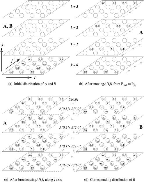
The cost-optimality condition for Cannon's algorithm is identical to that for the simple algorithm presented in Section 8.2.1. As in the simple algorithm, the isoefficiency function of Cannon's algorithm is Q(p^3/2).

8.2.3 The DNS Algorithm

The matrix multiplication algorithms presented so far use block 2-D partitioning of the input and the output matrices and use a maximum of n² processes for n x n matrices. As a result, these algorithms have a parallel run time of W(n) because there are Q(n³) operations in the serial algorithm. We now present a parallel algorithm based on partitioning intermediate data that can use up to n³ processes and that performs matrix multiplication in time Q(log n) by using W(n³/log n) processes. This algorithm is known as the DNS algorithm because it is due to Dekel, Nassimi, and Sahni.

We first introduce the basic idea, without concern for inter-process communication. Assume that n³ processes are available for multiplying two n x n matrices. These processes are arranged in a three-dimensional n x n x n logical array. Since the matrix multiplication algorithm performs n³ scalar multiplications, each of the n³ processes is assigned a single scalar multiplication. The processes are labeled according to their location in the array, and the multiplication A[i, k] x B[k, j] is assigned to process P_i,j,k (0 i, j, k < n). After each process performs a single multiplication, the contents of P_i,j,0, P_i,j,1, ..., P_i,j,n-1 are added to obtain C [i, j]. The additions for all C [i, j] can be carried out simultaneously in log n steps each. Thus, it takes one step to multiply and log n steps to add; that is, it takes time Q(log n) to multiply the n x n matrices by this algorithm.

We now describe a practical parallel implementation of matrix multiplication based on this idea. As Figure 8.4 shows, the process arrangement can be visualized as n planes of n x n processes each. Each plane corresponds to a different value of k. Initially, as shown in Figure 8.4(a), the matrices are distributed among the n² processes of the plane corresponding to k = 0 at the base of the three-dimensional process array. Process P_i,j,0 initially owns A[i, j] and B[i, j].

The vertical column of processes P_i,j,* computes the dot product of row A[i, *] and column B[*, j]. Therefore, rows of A and columns of B need to be moved appropriately so that each vertical column of processes P_i,j,* has row A[i, *] and column B[*, j]. More precisely, process P_i,j,k should have A[i, k] and B[k, j].

The communication pattern for distributing the elements of matrix A among the processes is shown in Figure 8.4(a)-(c). First, each column of A moves to a different plane such that the j th column occupies the same position in the plane corresponding to k = j as it initially did in the plane corresponding to k = 0. The distribution of A after moving A[i, j] from P_i,j,0 to P_i,j,j is shown in Figure 8.4(b). Now all the columns of A are replicated n times in their respective planes by a parallel one-to-all broadcast along the j axis. The result of this step is shown in Figure 8.4(c), in which the n processes P_i,0,j, P_i,1,j, ..., P_i,n-1,j receive a copy of A[i, j] from P_i,j,j. At this point, each vertical column of processes P_i,j,* has row A[i, *]. More precisely, process P_i,j,k has A[i, k].

For matrix B, the communication steps are similar, but the roles of i and j in process subscripts are switched. In the first one-to-one communication step, B[i, j] is moved from P_i,j,0 to P_i,j,i. Then it is broadcast from P_i,j,i among P_0,j,i, P_1,j,i, ..., P_n-1,j,i. The distribution of B after this one-to-all broadcast along the i axis is shown in Figure 8.4(d). At this point, each vertical column of processes P_i,j,* has column B[*, j]. Now process P_i,j,k has B[k, j], in addition to A[i, k].

After these communication steps, A[i, k] and B[k, j] are multiplied at P_i,j,k. Now each element C[i, j] of the product matrix is obtained by an all-to-one reduction along the k axis. During this step, process P_i,j,0 accumulates the results of the multiplication from processes P_i,j,1, ..., P_i,j,n-1. Figure 8.4 shows this step for C[0, 0].

The DNS algorithm has three main communication steps: (1) moving the columns of A and the rows of B to their respective planes, (2) performing one-to-all broadcast along the j axis for A and along the i axis for B, and (3) all-to-one reduction along the k axis. All these operations are performed within groups of n processes and take time Q(log n). Thus, the parallel run time for multiplying two n x n matrices using the DNS algorithm on n³ processes is Q(log n).

DNS Algorithm with Fewer than n³ Processes

The DNS algorithm is not cost-optimal for n³ processes, since its process-time product of Q(n³ log n) exceeds the Q(n³) sequential complexity of matrix multiplication. We now present a cost-optimal version of this algorithm that uses fewer than n³ processes. Another variant of the DNS algorithm that uses fewer than n³ processes is described in Problem 8.6.

Assume that the number of processes p is equal to q³ for some q < n. To implement the DNS algorithm, the two matrices are partitioned into blocks of size (n/q) x (n/q). Each matrix can thus be regarded as a q x q two-dimensional square array of blocks. The implementation of this algorithm on q³ processes is very similar to that on n³ processes. The only difference is that now we operate on blocks rather than on individual elements. Since 1 q n, the number of processes can vary between 1 and n³.

Performance Analysis The first one-to-one communication step is performed for both A and B, and takes time t_s + t_w(n/q)² for each matrix. The second step of one-to-all broadcast is also performed for both matrices and takes time t_s log q + t_w(n/q)² log q for each matrix. The final all-to-one reduction is performed only once (for matrix C)and takes time t_s log q + t_w(n/q)² log q. The multiplication of (n/q) x (n/q) submatrices by each process takes time (n/q)³. We can ignore the communication time for the first one-to-one communication step because it is much smaller than the communication time of one-to-all broadcasts and all-to-one reduction. We can also ignore the computation time for addition in the final reduction phase because it is of a smaller order of magnitude than the computation time for multiplying the submatrices. With these assumptions, we get the following approximate expression for the parallel run time of the DNS algorithm:

Since q = p^1/3, we get

Equation 8.16

The total cost of this parallel algorithm is n³ + t_s p log p + t_wn² p¹/³ log p. The isoefficiency function is Q(p(log p)³). The algorithm is cost-optimal for n³ = W(p(log p)³), or p = O(n³/(log n)³).