9.4 Quicksort

All the algorithms presented so far have worse sequential complexity than that of the lower bound for comparison-based sorting, Q(n log n). This section examines the quicksort algorithm, which has an average complexity of Q(n log n). Quicksort is one of the most common sorting algorithms for sequential computers because of its simplicity, low overhead, and optimal average complexity.

Quicksort is a divide-and-conquer algorithm that sorts a sequence by recursively dividing it into smaller subsequences. Assume that the n-element sequence to be sorted is stored in the array A[1...n]. Quicksort consists of two steps: divide and conquer. During the divide step, a sequence A[q...r] is partitioned (rearranged) into two nonempty subsequences A[q...s] and A[s + 1...r] such that each element of the first subsequence is smaller than or equal to each element of the second subsequence. During the conquer step, the subsequences are sorted by recursively applying quicksort. Since the subsequences A[q...s] and A[s + 1...r] are sorted and the first subsequence has smaller elements than the second, the entire sequence is sorted.

How is the sequence A[q...r] partitioned into two parts - one with all elements smaller than the other? This is usually accomplished by selecting one element x from A[q...r] and using this element to partition the sequence A[q...r] into two parts - one with elements less than or equal to x and the other with elements greater than x.Element x is called the pivot. The quicksort algorithm is presented in Algorithm 9.5. This algorithm arbitrarily chooses the first element of the sequence A[q...r] as the pivot. The operation of quicksort is illustrated in Figure 9.15.

Algorithm 9.5 The sequential quicksort algorithm.

1.   procedure QUICKSORT (A, q, r) 
2.   begin 
3.      if q < r then 
4.      begin 
5.         x := A[q]; 
6.         s := q; 
7.         for i := q + 1 to r do 
8.             if A[i]x then 
9.             begin 
10.               s := s + 1; 
11.               swap(A[s], A[i]); 
12.            end if 
13.        swap(A[q], A[s]); 
14.        QUICKSORT (A, q, s); 
15.        QUICKSORT (A, s + 1, r); 
16.     end if 
17.  end QUICKSORT 

The complexity of partitioning a sequence of size k is Q(k). Quicksort's performance is greatly affected by the way it partitions a sequence. Consider the case in which a sequence of size k is split poorly, into two subsequences of sizes 1 and k - 1. The run time in this case is given by the recurrence relation T(n) = T(n - 1) + Q(n), whose solution is T(n) = Q(n²). Alternatively, consider the case in which the sequence is split well, into two roughly equal-size subsequences of and elements. In this case, the run time is given by the recurrence relation T(n) = 2T(n/2) + Q(n), whose solution is T(n) = Q(n log n). The second split yields an optimal algorithm. Although quicksort can have O(n²) worst-case complexity, its average complexity is significantly better; the average number of compare-exchange operations needed by quicksort for sorting a randomly-ordered input sequence is 1.4n log n, which is asymptotically optimal. There are several ways to select pivots. For example, the pivot can be the median of a small number of elements of the sequence, or it can be an element selected at random. Some pivot selection strategies have advantages over others for certain input sequences.

9.4.1 Parallelizing Quicksort

Quicksort can be parallelized in a variety of ways. First, consider a naive parallel formulation that was also discussed briefly in Section 3.2.1 in the context of recursive decomposition. Lines 14 and 15 of Algorithm 9.5 show that, during each call of QUICKSORT, the array is partitioned into two parts and each part is solved recursively. Sorting the smaller arrays represents two completely independent subproblems that can be solved in parallel. Therefore, one way to parallelize quicksort is to execute it initially on a single process; then, when the algorithm performs its recursive calls (lines 14 and 15), assign one of the subproblems to another process. Now each of these processes sorts its array by using quicksort and assigns one of its subproblems to other processes. The algorithm terminates when the arrays cannot be further partitioned. Upon termination, each process holds an element of the array, and the sorted order can be recovered by traversing the processes as we will describe later. This parallel formulation of quicksort uses n processes to sort n elements. Its major drawback is that partitioning the array A[q ...r ] into two smaller arrays, A[q ...s] and A[s + 1 ...r ], is done by a single process. Since one process must partition the original array A[1 ...n], the run time of this formulation is bounded below by W(n). This formulation is not cost-optimal, because its process-time product is W(n²).

The main limitation of the previous parallel formulation is that it performs the partitioning step serially. As we will see in subsequent formulations, performing partitioning in parallel is essential in obtaining an efficient parallel quicksort. To see why, consider the recurrence equation T (n) = 2T (n/2) + Q(n), which gives the complexity of quicksort for optimal pivot selection. The term Q(n) is due to the partitioning of the array. Compare this complexity with the overall complexity of the algorithm, Q(n log n). From these two complexities, we can think of the quicksort algorithm as consisting of Q(log n) steps, each requiring time Q(n) - that of splitting the array. Therefore, if the partitioning step is performed in time Q(1), using Q(n) processes, it is possible to obtain an overall parallel run time of Q(log n), which leads to a cost-optimal formulation. However, without parallelizing the partitioning step, the best we can do (while maintaining cost-optimality) is to use only Q(log n) processes to sort n elements in time Q(n) (Problem 9.14). Hence, parallelizing the partitioning step has the potential to yield a significantly faster parallel formulation.

In the previous paragraph, we hinted that we could partition an array of size n into two smaller arrays in time Q(1) by using Q(n) processes. However, this is difficult for most parallel computing models. The only known algorithms are for the abstract PRAM models. Because of communication overhead, the partitioning step takes longer than Q(1) on realistic shared-address-space and message-passing parallel computers. In the following sections we present three distinct parallel formulations: one for a CRCW PRAM, one for a shared-address-space architecture, and one for a message-passing platform. Each of these formulations parallelizes quicksort by performing the partitioning step in parallel.

9.4.2 Parallel Formulation for a CRCW PRAM

We will now present a parallel formulation of quicksort for sorting n elements on an n-process arbitrary CRCW PRAM. Recall from Section 2.4.1 that an arbitrary CRCW PRAM is a concurrent-read, concurrent-write parallel random-access machine in which write conflicts are resolved arbitrarily. In other words, when more than one process tries to write to the same memory location, only one arbitrarily chosen process is allowed to write, and the remaining writes are ignored.

Executing quicksort can be visualized as constructing a binary tree. In this tree, the pivot is the root; elements smaller than or equal to the pivot go to the left subtree, and elements larger than the pivot go to the right subtree. Figure 9.16 illustrates the binary tree constructed by the execution of the quicksort algorithm illustrated in Figure 9.15. The sorted sequence can be obtained from this tree by performing an in-order traversal. The PRAM formulation is based on this interpretation of quicksort.

The algorithm starts by selecting a pivot element and partitioning the array into two parts - one with elements smaller than the pivot and the other with elements larger than the pivot. Subsequent pivot elements, one for each new subarray, are then selected in parallel. This formulation does not rearrange elements; instead, since all the processes can read the pivot in constant time, they know which of the two subarrays (smaller or larger) the elements assigned to them belong to. Thus, they can proceed to the next iteration.

The algorithm that constructs the binary tree is shown in Algorithm 9.6. The array to be sorted is stored in A[1...n] and process i is assigned element A[i]. The arrays leftchild[1...n] and rightchild[1...n] keep track of the children of a given pivot. For each process, the local variable parent_i stores the label of the process whose element is the pivot. Initially, all the processes write their process labels into the variable root in line 5. Because the concurrent write operation is arbitrary, only one of these labels will actually be written into root. The value A[root] is used as the first pivot and root is copied into parent_i for each process i . Next, processes that have elements smaller than A[parent_i] write their process labels into leftchild[parent_i], and those with larger elements write their process label into rightchild[parent_i]. Thus, all processes whose elements belong in the smaller partition have written their labels into leftchild[parent_i], and those with elements in the larger partition have written their labels into rightchild[parent_i]. Because of the arbitrary concurrent-write operations, only two values - one for leftchild[parent_i] and one for rightchild[parent_i] - are written into these locations. These two values become the labels of the processes that hold the pivot elements for the next iteration, in which two smaller arrays are being partitioned. The algorithm continues until n pivot elements are selected. A process exits when its element becomes a pivot. The construction of the binary tree is illustrated in Figure 9.17. During each iteration of the algorithm, a level of the tree is constructed in time Q(1). Thus, the average complexity of the binary tree building algorithm is Q(log n) as the average height of the tree is Q(log n) (Problem 9.16).

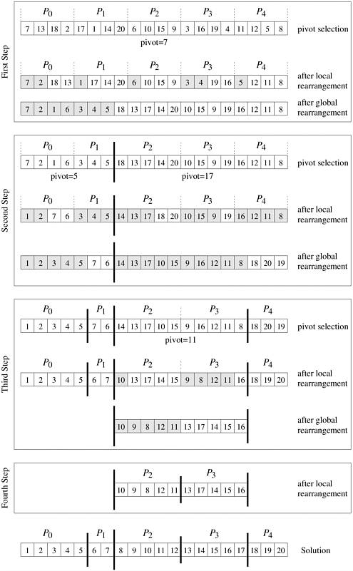
Algorithm 9.6 The binary tree construction procedure for the CRCW PRAM parallel quicksort formulation.

1.   procedure BUILD TREE (A[1...n]) 
2.   begin 
3.      for each process i do 
4.      begin 
5.         root := i; 
6.         parenti := root; 
7.         leftchild[i] := rightchild[i] := n + 1; 
8.      end for 
9.      repeat for each process i  r oot do 
10.     begin 
11.        if (A[i] < A[parenti]) or 
                (A[i]= A[parenti] and i <parenti) then 
12.        begin 
13.           leftchild[parenti] :=i ; 
14.           if i = leftchild[parenti] then exit 
15.           else parenti := leftchild[parenti]; 
16.        end for 
17.        else 
18.        begin 
19.           rightchild[parenti] :=i; 
20.           if i = rightchild[parenti] then exit 
21.           else parenti := rightchild[parenti]; 
22.        end else 
23.     end repeat 
24. end BUILD_TREE 

After building the binary tree, the algorithm determines the position of each element in the sorted array. It traverses the tree and keeps a count of the number of elements in the left and right subtrees of any element. Finally, each element is placed in its proper position in time Q(1), and the array is sorted. The algorithm that traverses the binary tree and computes the position of each element is left as an exercise (Problem 9.15). The average run time of this algorithm is Q(log n) on an n-process PRAM. Thus, its overall process-time product is Q(n log n), which is cost-optimal.

9.4.3 Parallel Formulation for Practical Architectures

We now turn our attention to a more realistic parallel architecture - that of a p-process system connected via an interconnection network. Initially, our discussion will focus on developing an algorithm for a shared-address-space system and then we will show how this algorithm can be adapted to message-passing systems.

Shared-Address-Space Parallel Formulation

The quicksort formulation for a shared-address-space system works as follows. Let A be an array of n elements that need to be sorted and p be the number of processes. Each process is assigned a consecutive block of n/p elements, and the labels of the processes define the global order of the sorted sequence. Let A_i be the block of elements assigned to process P_i .

The algorithm starts by selecting a pivot element, which is broadcast to all processes. Each process P_i, upon receiving the pivot, rearranges its assigned block of elements into two sub-blocks, one with elements smaller than the pivot S_i and one with elements larger than the pivot L_i. This local rearrangement is done in place using the collapsing the loops approach of quicksort. The next step of the algorithm is to rearrange the elements of the original array A so that all the elements that are smaller than the pivot (i.e., ) are stored at the beginning of the array, and all the elements that are larger than the pivot (i.e., ) are stored at the end of the array.

Once this global rearrangement is done, then the algorithm proceeds to partition the processes into two groups, and assign to the first group the task of sorting the smaller elements S, and to the second group the task of sorting the larger elements L . Each of these steps is performed by recursively calling the parallel quicksort algorithm. Note that by simultaneously partitioning both the processes and the original array each group of processes can proceed independently. The recursion ends when a particular sub-block of elements is assigned to only a single process, in which case the process sorts the elements using a serial quicksort algorithm.

The partitioning of processes into two groups is done according to the relative sizes of the S and L blocks. In particular, the first processes are assigned to sort the smaller elements S, and the rest of the processes are assigned to sort the larger elements L. Note that the 0.5 term in the above formula is to ensure that the processes are assigned in the most balanced fashion.

In order to globally rearrange the elements of A into the smaller and larger sub-arrays we need to know where each element of A will end up going at the end of that rearrangement. One way of doing this rearrangement is illustrated at the bottom of Figure 9.19. In this approach, S is obtained by concatenating the various S_i blocks over all the processes, in increasing order of process label. Similarly, L is obtained by concatenating the various L_i blocks in the same order. As a result, for process P_i, the j th element of its S_i sub-block will be stored at location , and the j th element of its L_i sub-block will be stored at location .

These locations can be easily computed using the prefix-sum operation described in Section 4.3. Two prefix-sums are computed, one involving the sizes of the S_i sub-blocks and the other the sizes of the L_i sub-blocks. Let Q and R be the arrays of size p that store these prefix sums, respectively. Their elements will be

Note that for each process P_i, Q_i is the starting location in the final array where its lower-than-the-pivot element will be stored, and R_i is the ending location in the final array where its greater-than-the-pivot elements will be stored. Once these locations have been determined, the overall rearrangement of A can be easily performed by using an auxiliary array A' of size n. These steps are illustrated in Figure 9.19. Note that the above definition of prefix-sum is slightly different from that described in Section 4.3, in the sense that the value that is computed for location Q_i (or R_i) does not include S_i (or L_i) itself. This type of prefix-sum is sometimes referred to as non-inclusive prefix-sum.

Analysis The complexity of the shared-address-space formulation of the quicksort algorithm depends on two things. The first is the amount of time it requires to split a particular array into the smaller-than- and the greater-than-the-pivot sub-arrays, and the second is the degree to which the various pivots being selected lead to balanced partitions. In this section, to simplify our analysis, we will assume that pivot selection always results in balanced partitions. However, the issue of proper pivot selection and its impact on the overall parallel performance is addressed in Section 9.4.4.

Given an array of n elements and p processes, the shared-address-space formulation of the quicksort algorithm needs to perform four steps: (i) determine and broadcast the pivot; (ii) locally rearrange the array assigned to each process; (iii) determine the locations in the globally rearranged array that the local elements will go to; and (iv) perform the global rearrangement. The first step can be performed in time Q(log p) using an efficient recursive doubling approach for shared-address-space broadcast. The second step can be done in time Q(n/p) using the traditional quicksort algorithm for splitting around a pivot element. The third step can be done in Q(log p) using two prefix sum operations. Finally, the fourth step can be done in at least time Q(n/p) as it requires us to copy the local elements to their final destination. Thus, the overall complexity of splitting an n-element array is Q(n/p) + Q(log p). This process is repeated for each of the two subarrays recursively on half the processes, until the array is split into p parts, at which point each process sorts the elements of the array assigned to it using the serial quicksort algorithm. Thus, the overall complexity of the parallel algorithm is:

Equation 9.8

The communication overhead in the above formulation is reflected in the Q(log² p) term, which leads to an overall isoefficiency of Q(p log² p). It is interesting to note that the overall scalability of the algorithm is determined by the amount of time required to perform the pivot broadcast and the prefix sum operations.

Message-Passing Parallel Formulation

The quicksort formulation for message-passing systems follows the general structure of the shared-address-space formulation. However, unlike the shared-address-space case in which array A and the globally rearranged array A' are stored in shared memory and can be accessed by all the processes, these arrays are now explicitly distributed among the processes. This makes the task of splitting A somewhat more involved.

In particular, in the message-passing version of the parallel quicksort, each process stores n/p elements of array A. This array is also partitioned around a particular pivot element using a two-phase approach. In the first phase (which is similar to the shared-address-space formulation), the locally stored array A_i at process P_i is partitioned into the smaller-than- and larger-than-the-pivot sub-arrays S_i and L_i locally. In the next phase, the algorithm first determines which processes will be responsible for recursively sorting the smaller-than-the-pivot sub-arrays (i.e., ) and which process will be responsible for recursively sorting the larger-than-the-pivot sub-arrays (i.e., ). Once this is done, then the processes send their S_i and L_i arrays to the corresponding processes. After that, the processes are partitioned into the two groups, one for S and one for L, and the algorithm proceeds recursively. The recursion terminates when each sub-array is assigned to a single process, at which point it is sorted locally.

The method used to determine which processes will be responsible for sorting S and L is identical to that for the shared-address-space formulation, which tries to partition the processes to match the relative size of the two sub-arrays. Let p_S and p_L be the number of processes assigned to sort S and L, respectively. Each one of the p_S processes will end up storing |S|/p_S elements of the smaller-than-the-pivot sub-array, and each one of the p_L processes will end up storing |L|/p_L elements of the larger-than-the-pivot sub-array. The method used to determine where each process P_i will send its S_i and L_i elements follows the same overall strategy as the shared-address-space formulation. That is, the various S_i (or L_i) sub-arrays will be stored in consecutive locations in S (or L) based on the process number. The actual processes that will be responsible for these elements are determined by the partition of S (or L) into p_S (or p_L) equal-size segments, and can be computed using a prefix-sum operation. Note that each process P_i may need to split its S_i (or L_i) sub-arrays into multiple segments and send each one to different processes. This can happen because its elements may be assigned to locations in S (or L) that span more than one process. In general, each process may have to send its elements to two different processes; however, there may be cases in which more than two partitions are required.

Analysis Our analysis of the message-passing formulation of quicksort will mirror the corresponding analysis of the shared-address-space formulation.

Consider a message-passing parallel computer with p processes and O (p) bisection bandwidth. The amount of time required to split an array of size n is Q(log p) for broadcasting the pivot element, Q(n/p) for splitting the locally assigned portion of the array, Q(log p) for performing the prefix sums to determine the process partition sizes and the destinations of the various S_i and L_i sub-arrays, and the amount of time required for sending and receiving the various arrays. This last step depends on how the processes are mapped on the underlying architecture and on the maximum number of processes that each process needs to communicate with. In general, this communication step involves all-to-all personalized communication (because a particular process may end-up receiving elements from all other processes), whose complexity has a lower bound of Q(n/p). Thus, the overall complexity for the split is Q(n/p) + Q(log p), which is asymptotically similar to that of the shared-address-space formulation. As a result, the overall runtime is also the same as in Equation 9.8, and the algorithm has a similar isoefficiency function of Q(p log² p).

9.4.4 Pivot Selection

In the parallel quicksort algorithm, we glossed over pivot selection. Pivot selection is particularly difficult, and it significantly affects the algorithm's performance. Consider the case in which the first pivot happens to be the largest element in the sequence. In this case, after the first split, one of the processes will be assigned only one element, and the remaining p - 1 processes will be assigned n - 1 elements. Hence, we are faced with a problem whose size has been reduced only by one element but only p - 1 processes will participate in the sorting operation. Although this is a contrived example, it illustrates a significant problem with parallelizing the quicksort algorithm. Ideally, the split should be done such that each partition has a non-trivial fraction of the original array.

One way to select pivots is to choose them at random as follows. During the i^th split, one process in each of the process groups randomly selects one of its elements to be the pivot for this partition. This is analogous to the random pivot selection in the sequential quicksort algorithm. Although this method seems to work for sequential quicksort, it is not well suited to the parallel formulation. To see this, consider the case in which a bad pivot is selected at some point. In sequential quicksort, this leads to a partitioning in which one subsequence is significantly larger than the other. If all subsequent pivot selections are good, one poor pivot will increase the overall work by at most an amount equal to the length of the subsequence; thus, it will not significantly degrade the performance of sequential quicksort. In the parallel formulation, however, one poor pivot may lead to a partitioning in which a process becomes idle, and that will persist throughout the execution of the algorithm.

If the initial distribution of elements in each process is uniform, then a better pivot selection method can be derived. In this case, the n/p elements initially stored at each process form a representative sample of all n elements. In other words, the median of each n/p-element subsequence is very close to the median of the entire n-element sequence. Why is this a good pivot selection scheme under the assumption of identical initial distributions? Since the distribution of elements on each process is the same as the overall distribution of the n elements, the median selected to be the pivot during the first step is a good approximation of the overall median. Since the selected pivot is very close to the overall median, roughly half of the elements in each process are smaller and the other half larger than the pivot. Therefore, the first split leads to two partitions, such that each of them has roughly n/2 elements. Similarly, the elements assigned to each process of the group that is responsible for sorting the smaller-than-the-pivot elements (and the group responsible for sorting the larger-than-the-pivot elements) have the same distribution as the n/2 smaller (or larger) elements of the original list. Thus, the split not only maintains load balance but also preserves the assumption of uniform element distribution in the process group. Therefore, the application of the same pivot selection scheme to the sub-groups of processes continues to yield good pivot selection.

Can we really assume that the n/p elements in each process have the same distribution as the overall sequence? The answer depends on the application. In some applications, either the random or the median pivot selection scheme works well, but in others neither scheme delivers good performance. Two additional pivot selection schemes are examined in Problems 9.20 and 9.21.